前言
写在前面
虽然这门课学习了机器学习的相关知识,但是只是基于sklearn包scikit-learn中文社区 进行调参,并没有手动实践机器学习的相关算法。只能说是对机器学习这门课有一个大概的初步认识,加之老师讲课的内容比较基础,关于机器学习的知识大多都是B站自学的。(其实就是上课没听过课而已)
书籍采用的是李航版本的《统计学习方法》,B站上有很多教程,所以不推荐硬啃书,看视频消化的更快。视频链接:十分钟机器学习
可能后期会自主编写相关机器学习的代码,从最基本的感知机开始……那都是后话了。
工具
老师推荐的是Spyder(其实Anaconda里面自带了),但是这里更加推荐的是Pycharm里面的Juypter。
配置Python环境
安装虚拟环境
1 conda create -n sklearn python=3.8
激活虚拟环境
安装包
1 2 3 4 5 6 7 8 9 10 11 conda install numpy conda install scipy conda install scikit-learn conda install matplotlib conda install seaborn conda install pandas
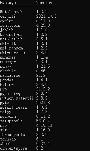
展示安装包
数据预处理与数据分析
导入库与数据
导入库
1 2 3 4 5 6 import numpy as npimport matplotlib.pyplot as pltimport pandas as pdimport seaborn as snsfrom scipy import statsfrom IPython.display import display
导入数据集
注:数据的excel文件需要放在.ipynb文件的同一目录下
1 2 data = pd.read_csv('train.csv' ) data
PassengerId
Survived
Pclass
Name
Sex
Age
SibSp
Parch
Ticket
Fare
Cabin
Embarked
0
1
0
3
Braund, Mr. Owen Harris
male
22.0
1
0
A/5 21171
7.2500
NaN
S
1
2
1
1
Cumings, Mrs. John Bradley (Florence Briggs Th...
female
38.0
1
0
PC 17599
71.2833
C85
C
2
3
1
3
Heikkinen, Miss. Laina
female
26.0
0
0
STON/O2. 3101282
7.9250
NaN
S
3
4
1
1
Futrelle, Mrs. Jacques Heath (Lily May Peel)
female
35.0
1
0
113803
53.1000
C123
S
4
5
0
3
Allen, Mr. William Henry
male
35.0
0
0
373450
8.0500
NaN
S
...
...
...
...
...
...
...
...
...
...
...
...
...
886
887
0
2
Montvila, Rev. Juozas
male
27.0
0
0
211536
13.0000
NaN
S
887
888
1
1
Graham, Miss. Margaret Edith
female
19.0
0
0
112053
30.0000
B42
S
888
889
0
3
Johnston, Miss. Catherine Helen "Carrie"
female
NaN
1
2
W./C. 6607
23.4500
NaN
S
889
890
1
1
Behr, Mr. Karl Howell
male
26.0
0
0
111369
30.0000
C148
C
890
891
0
3
Dooley, Mr. Patrick
male
32.0
0
0
370376
7.7500
NaN
Q
891 rows × 12 columns
概括性度量数据
PassengerId
Survived
Pclass
Age
SibSp
Parch
Fare
count
891.000000
891.000000
891.000000
714.000000
891.000000
891.000000
891.000000
mean
446.000000
0.383838
2.308642
29.699118
0.523008
0.381594
32.204208
std
257.353842
0.486592
0.836071
14.526497
1.102743
0.806057
49.693429
min
1.000000
0.000000
1.000000
0.420000
0.000000
0.000000
0.000000
25%
223.500000
0.000000
2.000000
20.125000
0.000000
0.000000
7.910400
50%
446.000000
0.000000
3.000000
28.000000
0.000000
0.000000
14.454200
75%
668.500000
1.000000
3.000000
38.000000
1.000000
0.000000
31.000000
max
891.000000
1.000000
3.000000
80.000000
8.000000
6.000000
512.329200
备份数据
数据处理
字符串数据处理判断标准:若字符串的重复率低于30%,则认定字符串与乘客存活无关
空缺数据处理判断标准:空缺率在20%以上的数据集无意义,空缺率在20%以下的数据集中的空缺数据可以用平均值代替
1 df.isnull().sum (axis=0 )/len (df)
PassengerId 0.000000
Survived 0.000000
Pclass 0.000000
Name 0.000000
Sex 0.000000
Age 0.198653
SibSp 0.000000
Parch 0.000000
Ticket 0.000000
Fare 0.000000
Cabin 0.771044
Embarked 0.002245
dtype: float64
性别处理
将男性编号为1,女性编号为0
1 2 3 4 5 def sex_value (sex ): if sex=='male' : return 1 else : return 0
1 df['Sex' ]=df['Sex' ].apply(lambda x:sex_value(x))
姓名处理
1 2 print ('姓名重复率:' )(len (df) - df['Name' ].unique().shape[0 ])/len (df)
姓名重复率:0.0
船票编号处理
1 2 print ('船票编号重复率:' )(len (df) - df['Ticket' ].unique().shape[0 ])/len (df)
船票编号重复率:0.2356902356902357
乘客乘船码头处理
乘客乘船码头重复率
1 2 print ('乘客登船码头重复率:' )(len (df) - df['Embarked' ].unique().shape[0 ])/len (df)
乘客登船码头重复率:0.9955106621773289
删去缺失数据
1 2 df = df.dropna(axis=0 ,subset=['Embarked' ]) df.reset_index(drop=True , inplace=True )
将字符串对应成编号
1 2 3 df['Embarked' ] =df['Embarked' ].replace('C' , 1 ) df['Embarked' ] =df['Embarked' ].replace('Q' , 2 ) df['Embarked' ] =df['Embarked' ].replace('S' , 3 )
年龄处理
随机森林回归填补缺失值
导入机器学习中的随机森林回归(RandomForestRegressor)方法
1 from sklearn.ensemble import RandomForestRegressor
不含缺失值的其他所有列
1 df_full=df.drop(labels=['Age' ,'PassengerId' ,'Name' ,'Ticket' ,'Cabin' ],axis=1 )
含缺失值的那一列
区别测试集与训练集
0 True
1 True
2 True
3 True
4 True
...
884 True
885 True
886 False
887 True
888 True
Name: Age, Length: 889, dtype: bool
0 False
1 False
2 False
3 False
4 False
...
884 False
885 False
886 True
887 False
888 False
Name: Age, Length: 889, dtype: bool
1 2 Xtrain = df_full[df_nan.notnull()] Ytrain = df_nan[df_nan.notnull()]
1 2 Ytest = df_nan[df_nan.isnull()] Xtest = df_full.iloc[Ytest.index]
随机森林训练及预测
1 2 3 rfc = RandomForestRegressor(n_estimators=100 ) rfc = rfc.fit(Xtrain, Ytrain) Ypredict = rfc.predict(Xtest)
预测结果四舍五入
1 Ypredict_round = Ypredict.round ()
填入预测数据
1 df_nan[df_nan.isnull()] = Ypredict_round
PassengerId
Survived
Pclass
Name
Sex
Age
SibSp
Parch
Ticket
Fare
Cabin
Embarked
0
1
0
3
Braund, Mr. Owen Harris
1
22.0
1
0
A/5 21171
7.2500
NaN
3
1
2
1
1
Cumings, Mrs. John Bradley (Florence Briggs Th...
0
38.0
1
0
PC 17599
71.2833
C85
1
2
3
1
3
Heikkinen, Miss. Laina
0
26.0
0
0
STON/O2. 3101282
7.9250
NaN
3
3
4
1
1
Futrelle, Mrs. Jacques Heath (Lily May Peel)
0
35.0
1
0
113803
53.1000
C123
3
4
5
0
3
Allen, Mr. William Henry
1
35.0
0
0
373450
8.0500
NaN
3
...
...
...
...
...
...
...
...
...
...
...
...
...
884
887
0
2
Montvila, Rev. Juozas
1
27.0
0
0
211536
13.0000
NaN
3
885
888
1
1
Graham, Miss. Margaret Edith
0
19.0
0
0
112053
30.0000
B42
3
886
889
0
3
Johnston, Miss. Catherine Helen "Carrie"
0
23.0
1
2
W./C. 6607
23.4500
NaN
3
887
890
1
1
Behr, Mr. Karl Howell
1
26.0
0
0
111369
30.0000
C148
1
888
891
0
3
Dooley, Mr. Patrick
1
32.0
0
0
370376
7.7500
NaN
2
889 rows × 12 columns
1 2 3 4 col_x = ['Pclass' ,'Sex' ,'Age' ,'SibSp' ,'Parch' ,'Fare' ,'Embarked' ] col_y = ['Survived' ] X = pd.DataFrame(df,columns = col_x) y=pd.DataFrame(df,columns = col_y)
测试集处理
1 2 3 data_predict = pd.read_csv('test.csv' ) df_predict = data_predict.copy() df_predict
PassengerId
Pclass
Name
Sex
Age
SibSp
Parch
Ticket
Fare
Cabin
Embarked
0
892
3
Kelly, Mr. James
male
34.5
0
0
330911
7.8292
NaN
Q
1
893
3
Wilkes, Mrs. James (Ellen Needs)
female
47.0
1
0
363272
7.0000
NaN
S
2
894
2
Myles, Mr. Thomas Francis
male
62.0
0
0
240276
9.6875
NaN
Q
3
895
3
Wirz, Mr. Albert
male
27.0
0
0
315154
8.6625
NaN
S
4
896
3
Hirvonen, Mrs. Alexander (Helga E Lindqvist)
female
22.0
1
1
3101298
12.2875
NaN
S
...
...
...
...
...
...
...
...
...
...
...
...
413
1305
3
Spector, Mr. Woolf
male
NaN
0
0
A.5. 3236
8.0500
NaN
S
414
1306
1
Oliva y Ocana, Dona. Fermina
female
39.0
0
0
PC 17758
108.9000
C105
C
415
1307
3
Saether, Mr. Simon Sivertsen
male
38.5
0
0
SOTON/O.Q. 3101262
7.2500
NaN
S
416
1308
3
Ware, Mr. Frederick
male
NaN
0
0
359309
8.0500
NaN
S
417
1309
3
Peter, Master. Michael J
male
NaN
1
1
2668
22.3583
NaN
C
418 rows × 11 columns
1 df_predict.isnull().sum (axis=0 )/len (df_predict)
PassengerId 0.000000
Pclass 0.000000
Name 0.000000
Sex 0.000000
Age 0.205742
SibSp 0.000000
Parch 0.000000
Ticket 0.000000
Fare 0.002392
Cabin 0.782297
Embarked 0.000000
dtype: float64
1 2 3 4 5 6 7 8 9 10 11 12 df_predict = df_predict.dropna(axis=0 ,subset=['Fare' ]) df_predict.reset_index(drop=True , inplace=True ) df_predict['Sex' ]=df_predict['Sex' ].apply(lambda x:sex_value(x)) df_predict['Embarked' ] =df_predict['Embarked' ].replace('C' , 1 ) df_predict['Embarked' ] =df_predict['Embarked' ].replace('Q' , 2 ) df_predict['Embarked' ] =df_predict['Embarked' ].replace('S' , 3 ) age_mean=df_predict['Age' ].mean() df_predict['Age' ]=df_predict['Age' ].fillna(age_mean) df_predict['Age' ]=df_predict['Age' ].round ()
1 X_predict = pd.DataFrame(df_predict,columns = col_x)
数据分析
统计量分析
计算均值、方差、标准差 (取了一些有意义的数据)
1 pd.DataFrame({"平均数" :X.mean(),"方差" :X.var(),"标准差" :X.std()}).T
Pclass
Sex
Age
SibSp
Parch
Fare
Embarked
平均数
2.311586
0.649044
29.534499
0.524184
0.382452
32.096681
2.535433
方差
0.696724
0.228042
189.760852
1.218164
0.650863
2469.841935
0.627403
标准差
0.834700
0.477538
13.775371
1.103705
0.806761
49.697504
0.792088
偏度与峰度
1 pd.DataFrame({'偏度' : X.skew(), '峰度' : X.kurt()},).T
Pclass
Sex
Age
SibSp
Parch
Fare
Embarked
偏度
-0.636998
-0.625625
0.417878
3.691058
2.745160
4.801440
-1.261367
峰度
-1.269437
-1.612225
0.378453
17.838972
9.750592
33.508477
-0.216100
协方差
Pclass
Sex
Age
SibSp
Parch
Fare
Embarked
Pclass
0.696724
0.050918
-4.453329
0.075226
0.011330
-22.740426
0.108880
Sex
0.050918
0.228042
0.965950
-0.061323
-0.095355
-4.270831
0.041729
Age
-4.453329
0.965950
189.760852
-4.765379
-2.344380
58.171717
-0.134675
SibSp
0.075226
-0.061323
-4.765379
1.218164
0.369119
8.824866
0.060234
Parch
0.011330
-0.095355
-2.344380
0.369119
0.650863
8.721729
0.025848
Fare
-22.740426
-4.270831
58.171717
8.824866
8.721729
2469.841935
-8.908691
Embarked
0.108880
0.041729
-0.134675
0.060234
0.025848
-8.908691
0.627403
相关矩阵
Pclass
Sex
Age
SibSp
Parch
Fare
Embarked
Pclass
1.000000
0.127741
-0.387303
0.081656
0.016824
-0.548193
0.164681
Sex
0.127741
1.000000
0.146840
-0.116348
-0.247508
-0.179958
0.110320
Age
-0.387303
0.146840
1.000000
-0.313430
-0.210950
0.084972
-0.012343
SibSp
0.081656
-0.116348
-0.313430
1.000000
0.414542
0.160887
0.068900
Parch
0.016824
-0.247508
-0.210950
0.414542
1.000000
0.217532
0.040449
Fare
-0.548193
-0.179958
0.084972
0.160887
0.217532
1.000000
-0.226311
Embarked
0.164681
0.110320
-0.012343
0.068900
0.040449
-0.226311
1.000000
图表分析
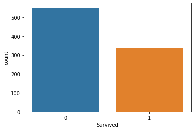
统计图
1 2 3 fig = plt.figure() sns.countplot(data=df, x='Survived' ) plt.show()
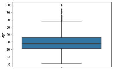
箱型图
1 2 3 fig = plt.figure() sns.boxplot(data=df, y='Age' ) plt.show()
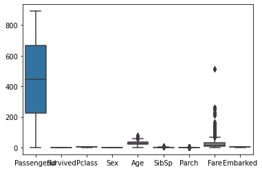
全体箱型图
1 2 3 fig = plt.figure() sns.boxplot(data=df) plt.show()
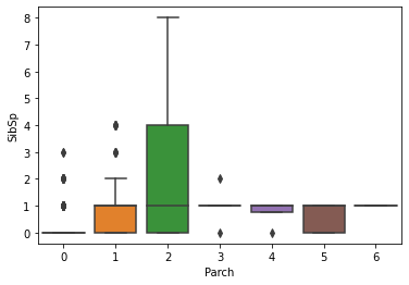
1 2 3 fig = plt.figure() sns.boxplot(data=df,y='SibSp' , x='Parch' ) plt.show()
散点图
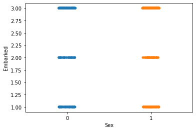
1 2 3 fig = plt.figure() sns.stripplot(data=df, x='Sex' , y='Embarked' ) plt.show()
直方图
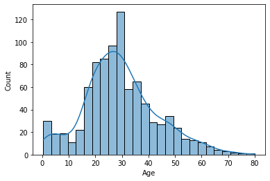
1 2 3 fig = plt.figure() sns.histplot(df, x='Age' , kde=True ) plt.show()
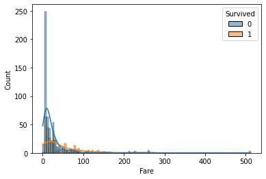
1 2 3 fig = plt.figure() sns.histplot(df, x='Fare' , hue='Survived' , kde=True ) plt.show()
散点图
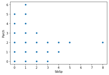
1 2 3 fig = plt.figure() sns.scatterplot(data=df, x='SibSp' , y='Parch' ) plt.show()
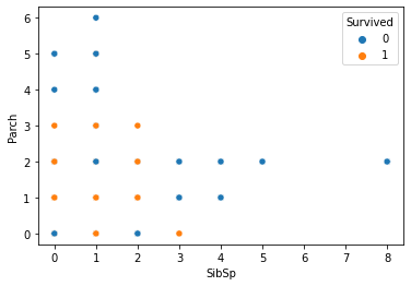
1 2 3 fig = plt.figure() sns.scatterplot(data=df, x='SibSp' , y='Parch' , hue='Survived' ) plt.show()
联合分布图
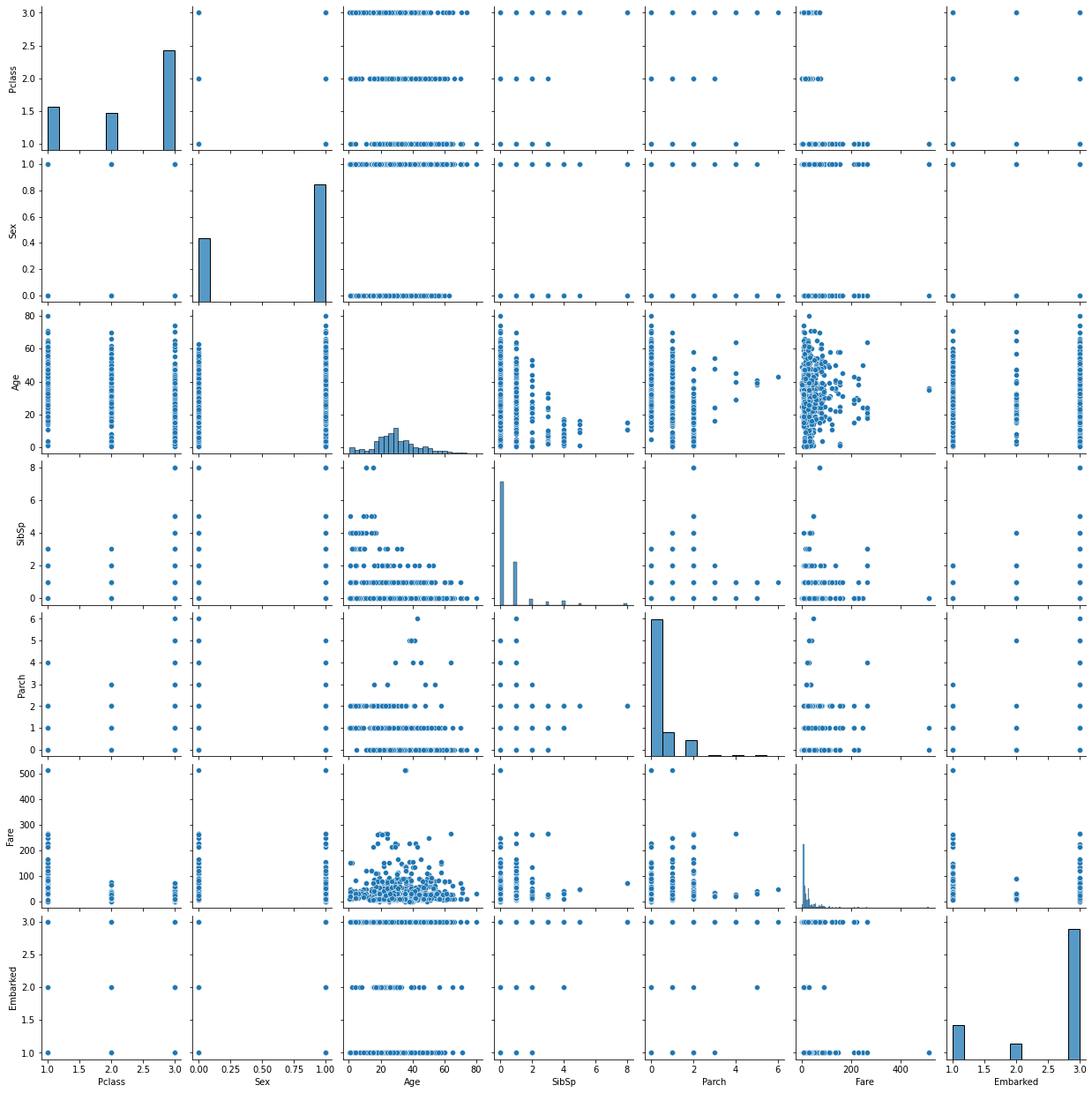
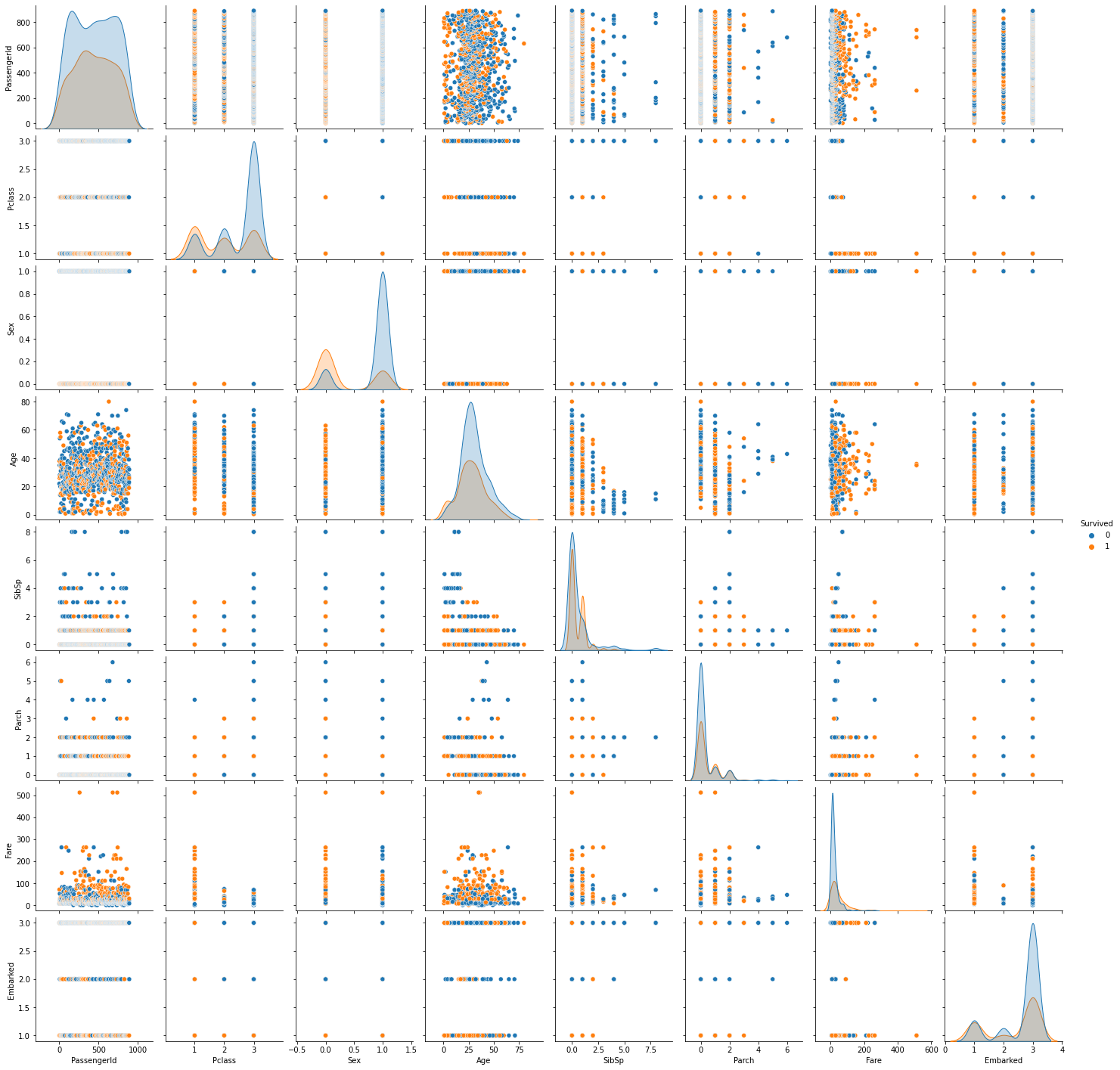
1 2 3 fig = plt.figure() sns.pairplot(X) plt.show()
<Figure size 432x288 with 0 Axes>
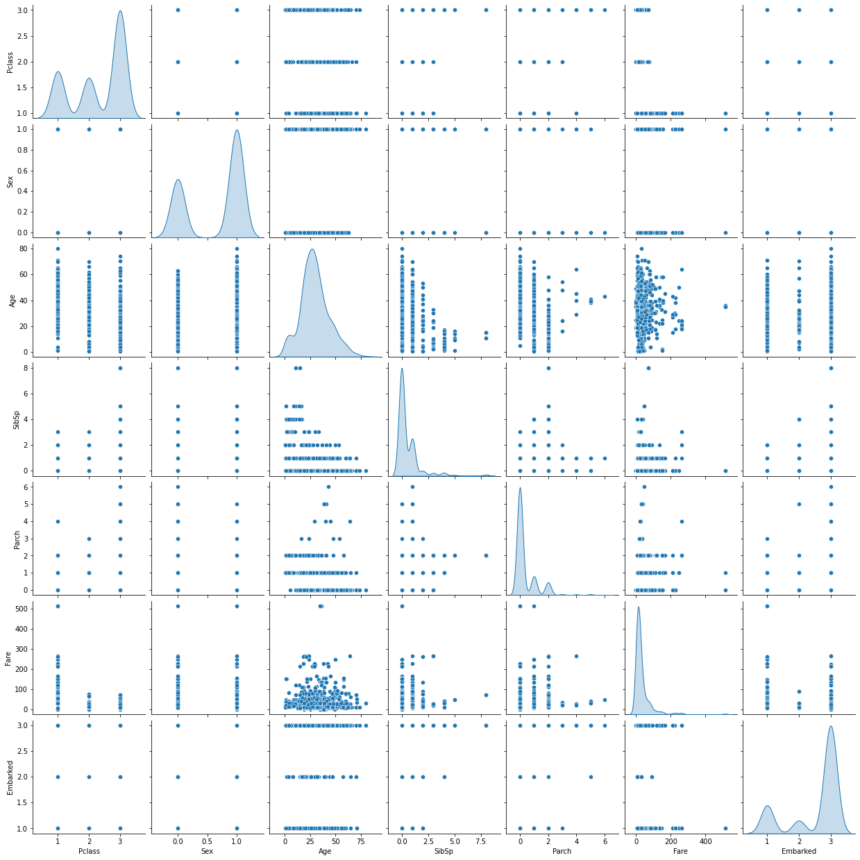
1 2 3 fig = plt.figure() sns.pairplot(X, diag_kind='kde' ) plt.show()
<Figure size 432x288 with 0 Axes>
1 2 3 fig = plt.figure() sns.pairplot(df, hue='Survived' , diag_kind='kde' ) plt.show()
<Figure size 432x288 with 0 Axes>
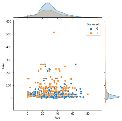
1 2 3 fig = plt.figure() g = sns.jointplot(data=df, x='Age' , y='Fare' , hue='Survived' ) plt.show()
<Figure size 432x288 with 0 Axes>
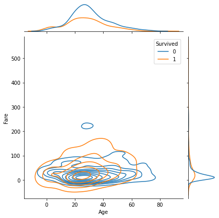
1 2 3 fig = plt.figure() sns.jointplot(data=df, x='Age' , y='Fare' , hue='Survived' , kind='kde' ) plt.show()
<Figure size 432x288 with 0 Axes>
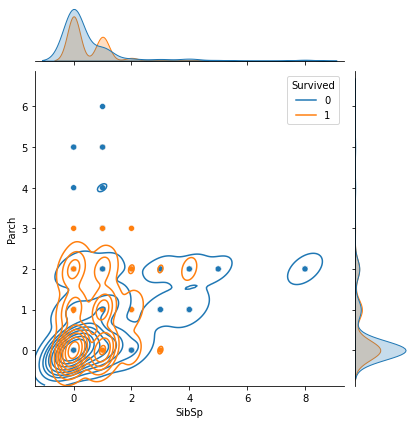
1 2 3 4 fig = plt.figure() g = sns.jointplot(data=df, x='SibSp' , y='Parch' , hue='Survived' ) g.plot_joint(sns.kdeplot) plt.show()
<Figure size 432x288 with 0 Axes>
核密度估计
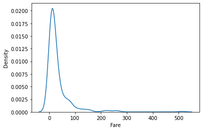
1 2 3 fig = plt.figure() sns.kdeplot(data=df, x='Fare' ) plt.show()
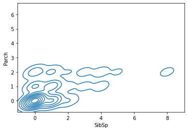
1 2 3 fig = plt.figure() sns.kdeplot(data=df, x='SibSp' , y='Parch' ) plt.show()
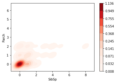
1 2 3 fig = plt.figure() sns.kdeplot(data=df, x='SibSp' , y='Parch' , fill=True , cbar=True , cmap='Reds' ) plt.show()
stats连续型随机变量的公共方法:
名称
备注
rvs
产生服从指定分布的随机数
cdf
累计分布函数
pdf
概率密度函数
sf
残存函数(1-CDF)
ppf
分位点函数(CDF的逆)
isf
逆残存函数(sf的逆)
fit
对一组随机取样进行拟合,最大似然估计方法找出最适合取样数据的概率密度函数系数。
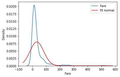
1 2 3 4 5 6 7 8 9 10 11 12 13 fig = plt.figure() ax = sns.kdeplot(data=df, x='Fare' , label='Fare' ) xmin, xmax = plt.xlim() x = np.linspace(xmin, xmax, 1000 ) mu, std = stats.norm.fit(df['Fare' ]) p = stats.norm.pdf(x, mu,std) ax.plot(x, p, 'r' , label='fit normal' ) ax.legend() plt.show() print (f'fitted mu: {mu} ' )print (f'fitted std: {std} ' )
fitted mu: 32.09668087739032
fitted std: 49.669545099689564
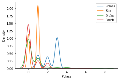
1 2 3 4 5 fig = plt.figure() for i in ['Pclass' , 'Sex' ,'SibSp' ,'Parch' ]: sns.kdeplot(data=df, x=i, label=i) plt.legend() plt.show()
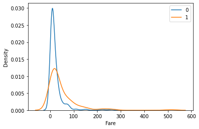
1 2 3 4 5 6 7 8 fig = plt.figure() s = df['Survived' ].astype("category" ) cates = s.cat.categories for cat in cates: df1 = df[df['Survived' ] == cat] sns.kdeplot(data=df1, x='Fare' , label=cat) plt.legend() plt.show()
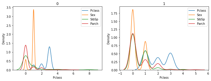
1 2 3 4 5 6 7 8 9 10 11 s = df['Survived' ].astype("category" ) cates = s.cat.categories fig,axs = plt.subplots(1 , len (cates), figsize=(len (cates) * 6 , 4 )) for col,cat in enumerate (cates): ax = axs[col] for i in ['Pclass' , 'Sex' ,'SibSp' ,'Parch' ]: df1 = df[df['Survived' ] == cat] sns.kdeplot(data=df1, x=i, label=i, ax=ax) ax.set_title(cat) ax.legend() plt.show()
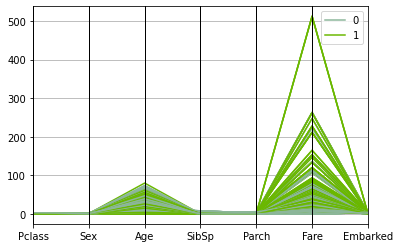
平行坐标系
1 2 pd.plotting.parallel_coordinates(pd.concat([X,y],axis=1 ), 'Survived' ) plt.show()
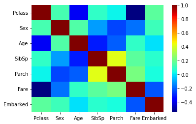
热力图
1 2 3 4 c = X.corr() display(c) sns.heatmap(c, cmap='jet' ) plt.show()
Pclass
Sex
Age
SibSp
Parch
Fare
Embarked
Pclass
1.000000
0.127741
-0.387303
0.081656
0.016824
-0.548193
0.164681
Sex
0.127741
1.000000
0.146840
-0.116348
-0.247508
-0.179958
0.110320
Age
-0.387303
0.146840
1.000000
-0.313430
-0.210950
0.084972
-0.012343
SibSp
0.081656
-0.116348
-0.313430
1.000000
0.414542
0.160887
0.068900
Parch
0.016824
-0.247508
-0.210950
0.414542
1.000000
0.217532
0.040449
Fare
-0.548193
-0.179958
0.084972
0.160887
0.217532
1.000000
-0.226311
Embarked
0.164681
0.110320
-0.012343
0.068900
0.040449
-0.226311
1.000000
分类模型
决策树模型
导入决策树模型
1 from sklearn import tree
决策树模型训练
1 from sklearn.model_selection import train_test_split
1 2 3 4 xtrain,xtest,ytrain,ytest = train_test_split(X, y,test_size=0.3 ) clf = tree.DecisionTreeClassifier() clf = clf.fit(xtrain,ytrain) print ('准确率:' , clf.score(xtest,ytest))
准确率: 0.7940074906367042
超参数优化
参数
说明
criterion {“gini”, “entropy”}, default=”gini” 这个参数是用来选择使用何种方法度量树的切分质量的。当criterion取值为“gini”时采用 基尼不纯度(Gini impurity)算法构造决策树,当criterion取值为 “entropy” 时采用信息增益( information gain)算法构造决策树.
splitter {“best”, “random”}, default=”best” 此参数决定了在每个节点上拆分策略的选择。支持的策略是“best” 选择“最佳拆分策略”, “random” 选择“最佳随机拆分策略”。
max_depth int, default=None 树的最大深度。如果取值为None,则将所有节点展开,直到所有的叶子都是纯净的或者直到所有叶子都包含少于min_samples_split个样本。
min_samples_split int or float, default=2 拆分内部节点所需的最少样本数: · 如果取值 int , 则将min_samples_split视为最小值。 · 如果为float,则min_samples_split是一个分数,而ceil(min_samples_split * n_samples)是每个拆分的最小样本数。 -注释 在版本0.18中更改:增加了分数形式的浮点值。
min_samples_leaf int or float, default=1 在叶节点处所需的最小样本数。 仅在任何深度的分裂点在左分支和右分支中的每个分支上至少留有min_samples_leaf个训练样本时,才考虑。 这可能具有平滑模型的效果,尤其是在回归中。 · 如果为int,则将min_samples_leaf视为最小值 · 如果为float,则min_samples_leaf是一个分数,而ceil(min_samples_leaf * n_samples)是每个节点的最小样本数。 - 注释: 在版本0.18中发生了更改:添加了分数形式的浮点值。
min_weight_fraction_leaf float, default=0.0 在所有叶节点处(所有输入样本)的权重总和中的最小加权分数。 如果未提供sample_weight,则样本的权重相等。
max_features int, float or {“auto”, “sqrt”, “log2”}, default=None 寻找最佳分割时要考虑的特征数量: - 如果为int,则在每次拆分时考虑max_features功能。 - 如果为float,则max_features是一个分数,而int(max_features * n_features)是每个分割处的特征数量。 - 如果为“auto”,则max_features = sqrt(n_features)。 - 如果为“sqrt”,则max_features = sqrt(n_features)。 - 如果为“log2”,则max_features = log2(n_features)。 - 如果为None,则max_features = n_features。 注意:直到找到至少一个有效的节点样本分区,分割的搜索才会停止,即使它需要有效检查的特征数量多于max_features也是如此。
random_state int, RandomState instance, default=None 此参数用来控制估计器的随机性。即使分割器设置为“最佳”,这些特征也总是在每个分割中随机排列。当max_features <n_features时,该算法将在每个拆分中随机选择max_features,然后再在其中找到最佳拆分。但是,即使max_features = n_features,找到的最佳分割也可能因不同的运行而有所不同。 就是这种情况,如果标准的改进对于几个拆分而言是相同的,并且必须随机选择一个拆分。 为了在拟合过程中获得确定性的行为,random_state必须固定为整数。 有关详细信息,请参见词汇表。
max_leaf_nodes int, default=None 优先以最佳方式生成带有max_leaf_nodes的树。 最佳节点定义为不纯度的相对减少。 如果为None,则叶节点数不受限制。
min_impurity_decrease float, default=0.0 如果节点分裂会导致不纯度的减少大于或等于该值,则该节点将被分裂。 加权不纯度减少方程如下: N_t / N * (impurity - N_t_R / N_t * right_impurity - N_t_L / N_t * left_impurity) 其中N是样本总数,N_t是当前节点上的样本数,N_t_L是左子节点中的样本数,N_t_R是右子节点中的样本数。 如果给sample_weight传了值,则N , N_t , N_t_R 和 N_t_L均指加权总和。 在 0.19 版新增 。
min_impurity_split float, default=0 树模型停止生长的阈值。如果节点的不纯度高于阈值,则该节点将分裂,否则为叶节点。 警告: 从版本0.19开始被弃用:min_impurity_split在0.19中被弃用,转而支持min_impurity_decrease。min_impurity_split的默认值在0.23中从1e-7更改为0,在0.25中将被删除。使用min_impurity_decrease代替。
class_weight dict, list of dict or “balanced”, default=None 以{class_label: weight}的形式表示与类别关联的权重。如果取值None,所有分类的权重为1。对于多输出问题,可以按照y的列的顺序提供一个字典列表。 注意多输出(包括多标签) ,应在其自己的字典中为每一列的每个类别定义权重。例如:对于四分类多标签问题, 权重应为[{0:1、1:1:1],{0:1、1:5},{0:1、1:1:1},{0:1、1: 1}],而不是[{1:1},{2:5},{3:1},{4:1}]。 “平衡”模式使用y的值自动将权重与输入数据中的类频率成反比地调整为n_samples /(n_classes * np.bincount(y))。 对于多输出,y的每一列的权重将相乘。 请注意,如果指定了sample_weight,则这些权重将与sample_weight(通过fit方法传递)相乘。
presort deprecated, default=’deprecated’ 此参数已弃用,并将在v0.24中删除。 注意:从0.22版开始已弃用。
ccp_alpha non-negative float, default=0.0 用于最小化成本复杂性修剪的复杂性参数。 将选择成本复杂度最大且小于ccp_alpha的子树。 默认情况下,不执行修剪。 有关详细信息,请参见最小成本复杂性修剪。
1 2 from sklearn.model_selection import StratifiedKFoldfrom sklearn.model_selection import GridSearchCV
1 2 3 4 5 6 7 8 9 10 11 12 clf = tree.DecisionTreeClassifier() parameters = { 'criterion' : ['entropy' , 'gini' ], 'max_leaf_nodes' : np.arange(2 , 9 ), 'max_depth' : [2 , 4 , 6 , 8 , 10 , 12 ], 'min_impurity_decrease' : [0 , 0.02 , 0.04 , 0.06 , 0.08 , 0.1 ], } skf = StratifiedKFold(n_splits=100 , shuffle=True ) clf_search = GridSearchCV(clf, parameters, cv=skf, scoring='accuracy' , n_jobs=-1 ) clf_search.fit(X, y) print ('最优参数:' ,clf_search.best_params_)print ('最优分数:' ,clf_search.best_score_)
最优参数: {'criterion': 'entropy', 'max_depth': 4, 'max_leaf_nodes': 8, 'min_impurity_decrease': 0}
最优分数: 0.8226388888888888
决策树模型平均准确度
1 from sklearn.model_selection import cross_val_score
1 2 3 scores = cross_val_score(clf_search.best_estimator_, X, y, cv=6 ) print ('平均得分:' , np.mean(scores))print ('得分:' , scores)
平均得分: 0.8155420521192333
得分: [0.79865772 0.81081081 0.85810811 0.78378378 0.7972973 0.84459459]
画图
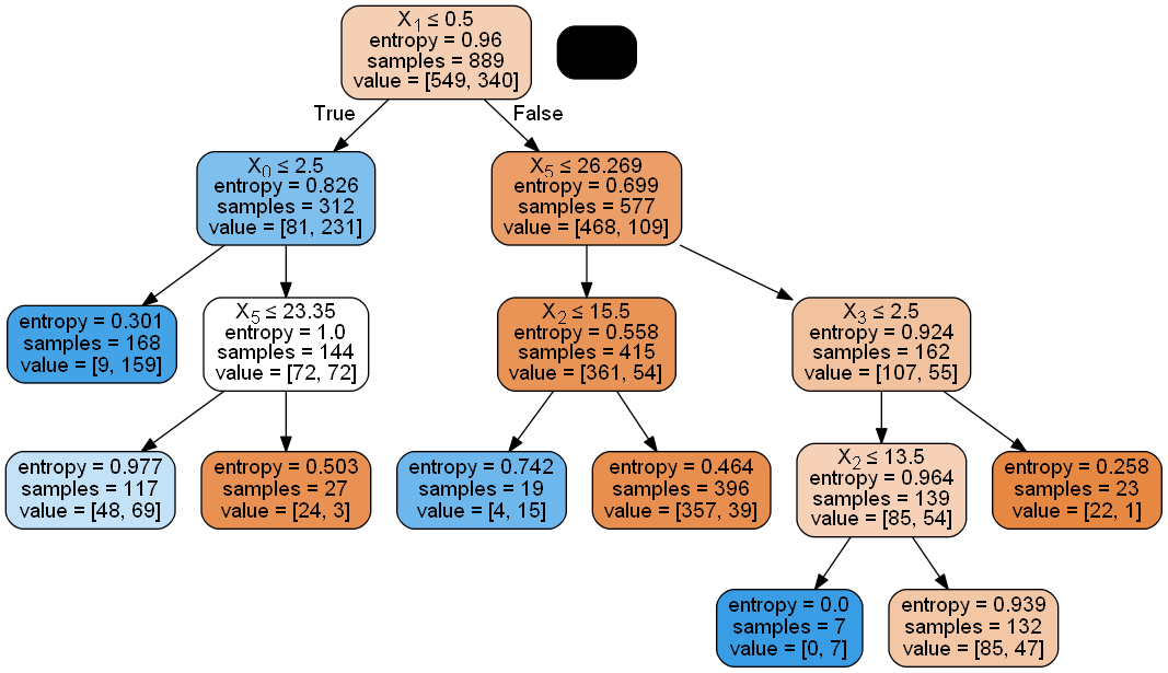
1 2 from IPython.display import Imageimport pydotplus
1 2 3 4 clf = clf.fit(X,y) dot_data = tree.export_graphviz(clf_search.best_estimator_,filled=True , rounded=True ,special_characters=True ) graph = pydotplus.graph_from_dot_data(dot_data) Image(graph.create_png())
测试集预测
1 2 import openpyxlypred = clf_search.best_estimator_.predict(X_predict)
输出预测结果
1 2 3 4 5 ytestId = pd.DataFrame(df_predict,columns = ['PassengerId' ]) ytest=pd.DataFrame(ypred) ytest=ytest.rename(columns={"Survived" :'PredictSurvived' }) result=ytestId.join(ytest) result.to_excel('决策树预测.xlsx' )
人工神经网络
导入模型
1 from sklearn.neural_network import MLPClassifier
标准化
1 from sklearn.preprocessing import StandardScaler
1 2 3 scaler = StandardScaler() scaler.fit(X) X_scaler = scaler.transform(X)
人工神经网络模型训练
1 from sklearn.model_selection import train_test_split
1 2 3 4 X_train,X_test,Y_train,Y_test=train_test_split(X_scaler,y,test_size=0.3 ) mlp = MLPClassifier() mlp = mlp.fit(X_train,Y_train) print ('准确率:' , mlp.score(X_test,Y_test))
准确率: 0.7865168539325843
超参数优化
参数
说明
hidden_layer_sizes tuple, length = n_layers - 2, default=(100,) 第i个元素代表第i个隐藏层中的神经元数量。
activation {‘identity’, ‘logistic’, ‘tanh’, ‘relu’}, default=’relu’ 隐藏层的激活函数。 - ‘identity’,无操作激活,用于实现线性瓶颈,返回f(x)= x - ‘logistic’,logistic Sigmoid函数,返回f(x)= 1 / (1 + exp(x))。 - ‘tanh’,双曲tan函数,返回f(x)= tanh(x)。 - ‘relu’,整流线性单位函数,返回f(x)= max(0,x)
solver {‘lbfgs’, ‘sgd’, ‘adam’}, default=’adam’ 权重优化的求解器。 - “ lbfgs”是quasi-Newton方法族的优化程序。 - “ sgd”是指随机梯度下降。 - “ adam”是指Kingma,Diederik和Jimmy Ba提出的基于随机梯度的优化器 注意:就训练时间和验证准确率而言,默认求解器“ adam”在相对较大的数据集(具有数千个训练样本或更多)上的效果很好。但是,对于小型数据集,“ lbfgs”可以收敛得更快并且性能更好。
alpha float, default=0.0001 L2惩罚(正则项)参数。
batch_size int, default=’auto’ 随机优化器的小批次的大小。如果求解器为“ lbfgs”,则分类器将不使用小批次批处理。设为“自动”时,batch_size=min(200, n_samples)
learning_rate {‘constant’, ‘invscaling’, ‘adaptive’}, default=’constant’ 权重更新的学习速率表。 - ’ constant ‘是一个恒定的学习速率,由’ learning_rate_init '给出。 - “invscaling”通过使用“power_t”的缩放逆指数,逐步降低在每个时间步长“t”上的学习率。effective_learning_rate = learning_rate_init / pow(t, power_t) - 只要训练损失持续减少,‘adaptive’将学习率保持在‘learning_rate_init’不变。每次连续两个epoch不能减少至少tol的训练损失,或者如果“early_stop”开启,不能增加至少tol的验证分数,则当前学习率要除以5。 仅在solver='sgd'时使用。
learning_rate_init double, default=0.001 使用的初始学习率。它控制更新权重的步长。仅在Solver ='sgd’或’adam’时使用。
power_t double, default=0.5 反比例学习率的指数。当learning_rate设置为“ invscaling”时,它用于更新有效学习率。仅在Solver ='sgd’时使用。
max_iter int, default=200 最大迭代次数。求解器迭代直到收敛(由“ tol”决定)或这个迭代次数。对于随机求解器(“ sgd”,“ adam”),请注意,这决定时期数(每个数据点将使用多少次),而不是梯度步数。
shuffle bool, default=True 是否在每次迭代中对样本进行打乱。仅在Solver ='sgd’或’adam’时使用。
random_state int, RandomState instance, default=None 决定用于权重和偏差初始化的随机数生成,如果使用了提前停止,则切分测试集和训练集,并在solver ='sgd’或’adam’时批量采样。在多个函数调用之间传递一个int值以获得可重复的结果。请参阅词汇表 。
tol float, default=1e-4 优化公差。当n_iter_no_change连续迭代的损失或分数没有通过至少tol得到改善时,除非将learning_rate设置为‘adaptive’,否则将认为达到收敛并停止训练。
verbose bool, default=False 是否将进度消息打印到标准输出。
warm_start bool, default=False 设置为True时,请重用上一个调用的解决方案以拟合初始化,否则,只需擦除以前的解决方案即可。请参阅词汇表 。
momentum float, default=0.9 梯度下降更新的动量。应该在0到1之间。仅在solver ='sgd’时使用。
nesterovs_momentum boolean, default=True 是否使用内Nesterov的动量。仅在Solver ='sgd’且momentum> 0时使用。
early_stopping bool, default=False 当验证准确率没有提高时,是否使用提前停止来终止训练。如果设置为true,它将自动预留10%的训练数据作为验证,并在n_iter_no_change连续几个时期,验证准确率没有提高至少tol时终止训练 。除多标签设置外,这个切分是分层的。仅在Solver ='sgd’或’adam’时有效
validation_fraction float, default=0.1 预留的训练数据比例作为提前停止的验证集。必须在0到1之间。仅当early_stopping为True时使用
beta_1 float, default=0.9 adam第一矩向量估计的指数衰减率,应在[0,1)范围内。仅在solver ='adam’时使用
beta_2 float, default=0.999 adam第二矩向量估计的指数衰减率,应在[0,1)范围内。仅在solver ='adam’时使用
epsilon float, default=1e-8 adam中数值稳定性的值。仅在solver ='adam’时使用
n_iter_no_change int, default=10 不满足tol改进的最大时期数。仅在Solver ='sgd’或’adam’时有效 0.20版中的新功能。
max_fun int, default=15000 仅在Solver ='lbfgs’时使用。损失函数调用的最大次数。求解器迭代直到收敛(由“ tol”确定),迭代次数达到max_iter或这个损失函数调用的次数。请注意,损失函数调用的次数将大于或等于MLPClassifier的迭代次数。 0.22版中的新功能。
1 from sklearn.model_selection import StratifiedShuffleSplit,GridSearchCV
1 2 3 4 5 6 7 8 9 10 11 mlp = MLPClassifier() parameters = [ {'activation' : ['logistic' , 'relu' , 'tanh' ],'alpha' : np.logspace(-5 , 3 , 5 ),'hidden_layer_sizes' : [ (100 ,), (120 ,), (140 ,), (160 ,), (180 ,), (200 ,)]}, {'activation' : ['relu' , 'tanh' ],'alpha' : np.logspace(-5 , 3 , 5 ),'hidden_layer_sizes' : [ (100 ,100 ), (120 ,120 ), (140 ,140 ), (160 ,160 ), (180 ,180 ), (200 ,200 )]}, {'activation' : ['relu' ],'alpha' : np.logspace(-5 , 3 , 5 ),'hidden_layer_sizes' : [ (100 ,100 ,100 ), (120 ,120 ,120 ), (140 ,140 ,140 ), (160 ,160 ,160 ), (180 ,180 ,180 ), (200 ,200 ,200 )]} ] skf = StratifiedShuffleSplit(n_splits = 20 , test_size=0.2 , random_state=1 ) mlp_search = GridSearchCV(mlp, parameters, cv=skf, scoring='accuracy' , n_jobs=-1 ) mlp_search.fit(X_scaler, y) print ('最优参数:' ,mlp_search.best_params_)print ('最优分数:' ,mlp_search.best_score_)
最优参数: {'activation': 'relu', 'alpha': 0.001, 'hidden_layer_sizes': (140,)}
最优分数: 0.8384831460674158
多指标评估
1 2 3 from sklearn.metrics import accuracy_scorefrom sklearn.metrics import make_scorerfrom sklearn.model_selection import cross_validate
1 2 3 4 scoring = {'accuracy' : make_scorer(accuracy_score),'prec' : 'precision' } cv_results = cross_validate(mlp_search.best_estimator_.fit(X_scaler, y), X_scaler, y, cv=5 , scoring=scoring) print (cv_results)
{'fit_time': array([0.80034709, 0.7290976 , 0.75559878, 0.75425696, 0.73791957]), 'score_time': array([0.00095391, 0.00199413, 0.00202894, 0.00202847, 0.0009973 ]), 'test_accuracy': array([0.82022472, 0.82022472, 0.84269663, 0.80337079, 0.86440678]), 'test_prec': array([0.82142857, 0.82142857, 0.84482759, 0.85106383, 0.84375 ])}
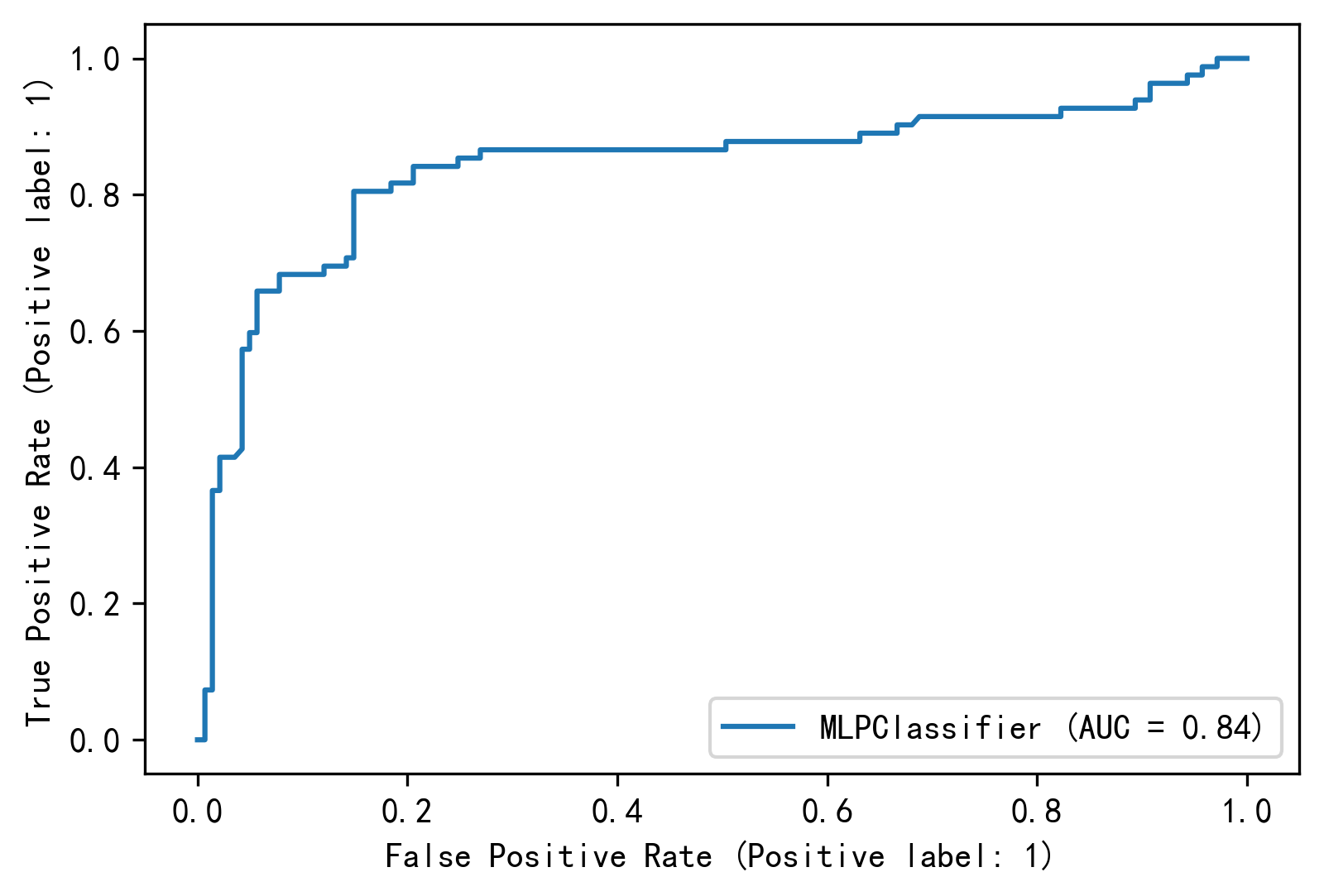
绘制ROC曲线
1 2 3 4 5 from sklearn.metrics import plot_roc_curveimport matplotlib.pyplot as pltplt.rcParams['figure.dpi' ] = 300 plt.rcParams['font.sans-serif' ] = ['SimHei' ] plt.rcParams['axes.unicode_minus' ] = False
1 2 3 4 5 X_train, X_test, y_train, y_test = train_test_split(X_scaler, y, random_state=42 ) mlp_search.best_estimator_.fit(X_train, y_train) roc_disp = plot_roc_curve(mlp_search.best_estimator_, X_test, y_test) plt.show()
测试集预测
1 2 3 4 5 scaler_predict = StandardScaler() scaler_predict.fit(X_predict) X_predict_scaler = scaler_predict.transform(X_predict) ypred = mlp_search.best_estimator_.predict(X_predict_scaler) ypred
array([0, 0, 0, 0, 0, 0, 0, 0, 1, 0, 0, 0, 1, 0, 1, 1, 0, 0, 0, 0, 0, 1,
1, 1, 1, 0, 1, 0, 0, 0, 0, 0, 0, 0, 1, 0, 0, 1, 0, 0, 0, 0, 0, 1,
1, 0, 0, 0, 1, 0, 0, 0, 1, 1, 0, 0, 0, 0, 0, 1, 0, 0, 0, 1, 1, 1,
1, 0, 0, 1, 1, 0, 0, 1, 1, 0, 0, 1, 0, 1, 1, 1, 0, 0, 0, 0, 0, 1,
0, 1, 0, 0, 1, 0, 1, 0, 1, 0, 1, 0, 1, 0, 0, 0, 1, 0, 0, 0, 0, 0,
0, 0, 1, 1, 1, 0, 0, 1, 0, 1, 1, 0, 1, 0, 0, 1, 0, 0, 0, 0, 0, 0,
0, 0, 0, 0, 0, 0, 1, 0, 0, 1, 0, 0, 0, 0, 0, 0, 0, 0, 1, 0, 0, 0,
0, 1, 1, 0, 1, 0, 1, 1, 0, 0, 0, 0, 0, 1, 1, 0, 0, 0, 0, 0, 1, 1,
0, 1, 1, 0, 1, 1, 0, 1, 0, 1, 0, 0, 0, 0, 0, 0, 0, 1, 0, 1, 1, 0,
0, 0, 1, 0, 1, 0, 1, 0, 0, 1, 0, 0, 0, 0, 1, 0, 0, 0, 0, 1, 0, 1,
0, 1, 0, 1, 0, 0, 0, 0, 0, 1, 1, 0, 0, 1, 0, 0, 0, 1, 1, 1, 1, 0,
0, 0, 0, 1, 0, 1, 1, 1, 0, 0, 0, 0, 0, 0, 0, 1, 0, 0, 0, 1, 1, 0,
0, 0, 0, 0, 0, 0, 0, 1, 0, 0, 1, 0, 0, 0, 0, 1, 1, 0, 1, 1, 0, 0,
0, 0, 0, 0, 0, 0, 0, 0, 0, 1, 0, 0, 0, 0, 0, 0, 0, 0, 1, 0, 1, 0,
0, 0, 0, 0, 0, 1, 1, 0, 0, 0, 0, 0, 0, 0, 0, 1, 0, 1, 0, 0, 0, 1,
0, 0, 1, 0, 0, 0, 0, 0, 0, 0, 0, 0, 1, 0, 1, 0, 0, 0, 1, 1, 0, 0,
0, 1, 0, 1, 0, 0, 0, 0, 1, 1, 0, 1, 0, 0, 1, 1, 0, 0, 1, 0, 0, 1,
1, 0, 0, 0, 0, 0, 0, 0, 0, 0, 1, 0, 0, 0, 0, 0, 1, 1, 0, 0, 1, 0,
1, 0, 0, 1, 0, 1, 1, 1, 1, 0, 0, 0, 1, 0, 1, 0, 0, 1, 0, 0, 0],
dtype=int64)
输出预测结果
1 2 3 4 5 ytestId = pd.DataFrame(df_predict, columns=['PassengerId' ]) ytest = pd.DataFrame(ypred) ytest = ytest.rename(columns={"Survived" : 'PredictSurvived' }) result = ytestId.join(ytest) result.to_excel('神经网络预测.xlsx' )
支持向量机
导入模型
支持向量机模型训练
1 2 from sklearn.model_selection import train_test_splitfrom sklearn.pipeline import make_pipeline
1 2 3 4 X_train,X_test,Y_train,Y_test=train_test_split(X,y,test_size=0.3 ) svms = make_pipeline(StandardScaler(), svm.SVC()) svms = svms.fit(X_train,Y_train) print ('准确率:' , svms.score(X_test,Y_test))
准确率: 0.7902621722846442
超参数优化
参数
说明
C 浮点数,默认= 1.0 正则化参数。正则化的强度与C成反比。必须严格为正。此惩罚系数是l2惩罚系数的平方
kernel {‘linear’, ‘poly’, ‘rbf’, ‘sigmoid’, ‘precomputed’}, 默认=’rbf’ 指定算法中使用的内核类型。它必须是“linear”,“poly”,“rbf”,“sigmoid”,“precomputed”或者“callable”中的一个。如果没有给出,将默认使用“rbf”。如果给定了一个可调用函数,则用它来预先计算核矩阵。该矩阵应为形状数组(n_samples,n_samples)
degree 整数型,默认=3 多项式核函数的次数(’ poly ')。将会被其他内核忽略。
gamma 浮点数或者{‘scale’, ‘auto’} , 默认=’scale’ 核系数包含‘rbf’, ‘poly’ 和‘sigmoid’ 如果gamma=‘scale’(默认),则它使用1 / (n_features * X.var())作为gamma的值,如果是auto,则使用1 / n_features。 在0.22版本有改动:默认的gamma从“auto”改为“scale”。
coef0 浮点数,默认=0.0 核函数中的独立项。它只在’ poly ‘和’ sigmoid '中有意义。
shrinking 布尔值,默认=True 是否使用缩小启发式,参见[使用指南](http://scikit-learn.org.cn/view/83.html#1.4.5 实用技巧)
probability 布尔值,默认=False 是否启用概率估计。必须在调用fit之前启用此参数,因为该方法内部使用5折交叉验证,因此会减慢该方法的速度,并且predict_proba可能与dict不一致。更多信息请阅读[使用指南](http://scikit-learn.org.cn/view/83.html#1.4.1 分类)
tol 浮点数,默认=1e-3 残差收敛条件。
cache_size 浮点数,默认=200 指定内核缓存的大小(以MB为单位)。
class_weight {dict, ‘balanced’}, 默认=None 在SVC中,将类i的参数C设置为class_weight [i] * C。如果没有给出值,则所有类都将设置为单位权重。“balanced”模式使用y的值自动将权重与类频率成反比地调整为n_samples / (n_classes * np.bincount(y))
verbose 布尔值,默认=False 是否启用详细输出。请注意,此参数针对liblinear中运行每个进程时设置,如果启用,则可能无法在多线程上下文中正常工作。
max_iter 整数型,默认=-1 对求解器内的迭代进行硬性限制,或者为-1(无限制时)。
decision_function_shape {‘ovo’, ‘ovr’}, 默认=’ovr’ 是否要将返回形状为(n_samples, n_classes)的one-vs-rest (‘ovr’)决策函数应用于其他所有分类器,而在多类别划分中始终使用one-vs-one (‘ovo’),对于二进制分类,将忽略该参数。 在版本0.19中进行了更改:默认情况下Decision_function_shape为ovr。 0.17版中的新功能:推荐使用Decision_function_shape =‘ovr’。 在0.17版中进行了更改:不建议使用Decision_function_shape ='ovo’和None。
break_ties bool, default=False 如果为true,decision_function_shape =‘ovr’,并且类数> 2,则预测将根据Decision_function的置信度值打破平局;否则,返回绑定类中的第一类。请注意,与简单的预测相比,打破平局的计算成本较高。 这是0.22版中的新功能。
random_state 整数型或RandomState的实例,默认=None 控制用于数据抽取时的伪随机数生成。当probability为False时将忽略该参数。在多个函数调用之间传递可重复输出的整数值。请参阅词汇表 。
1 2 3 from sklearn.model_selection import StratifiedShuffleSplitfrom sklearn.model_selection import GridSearchCVfrom sklearn.preprocessing import StandardScaler
1 2 3 scaler = StandardScaler() scaler.fit(X) X_scaler = scaler.transform(X)
1 2 3 4 5 6 7 8 9 10 11 12 svms = svm.SVC() parameters = { 'kernel' : ('linear' , 'poly' , 'rbf' , 'sigmoid' ), 'C' : [0.01 ,0.1 ,1 ,10 ,100 ], } skf = StratifiedShuffleSplit(n_splits = 20 , test_size=0.2 , random_state=1 ) svm_search = GridSearchCV(svms, parameters, cv=skf) svm_search.fit(X_scaler, y) print ('最优参数:' ,svm_search.best_params_)print ('最优分数:' ,svm_search.best_score_)
最优参数: {'C': 1, 'kernel': 'rbf'}
最优分数: 0.8294943820224718
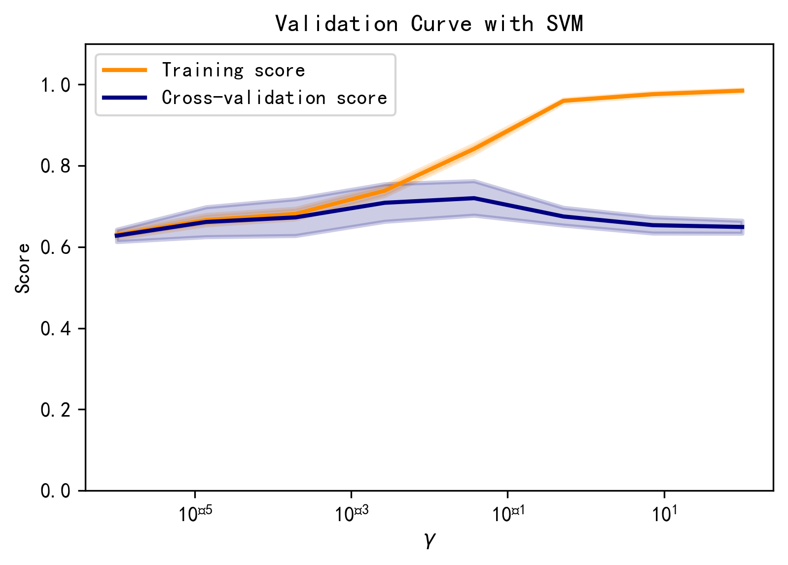
绘制验证曲线
1 from sklearn.model_selection import validation_curve
1 2 3 4 5 6 7 8 9 10 11 12 13 14 15 16 17 18 19 20 21 22 23 24 param_range = np.logspace(-6 , 2 , 8 ) train_scores, test_scores = validation_curve(svm.SVC(), X, y, param_name="gamma" ,param_range=param_range, scoring="accuracy" , n_jobs=1 ) train_scores_mean = np.mean(train_scores, axis=1 ) train_scores_std = np.std(train_scores, axis=1 ) test_scores_mean = np.mean(test_scores, axis=1 ) test_scores_std = np.std(test_scores, axis=1 ) plt.title("Validation Curve with SVM" ) plt.xlabel(r"$\gamma$" ) plt.ylabel("Score" ) plt.ylim(0.0 , 1.1 ) lw = 2 plt.semilogx(param_range, train_scores_mean, label="Training score" , color="darkorange" , lw=lw) plt.fill_between(param_range, train_scores_mean - train_scores_std, train_scores_mean + train_scores_std, alpha=0.2 , color="darkorange" , lw=lw) plt.semilogx(param_range, test_scores_mean, label="Cross-validation score" , color="navy" , lw=lw) plt.fill_between(param_range, test_scores_mean - test_scores_std, test_scores_mean + test_scores_std, alpha=0.2 , color="navy" , lw=lw) plt.legend(loc="best" ) plt.show()
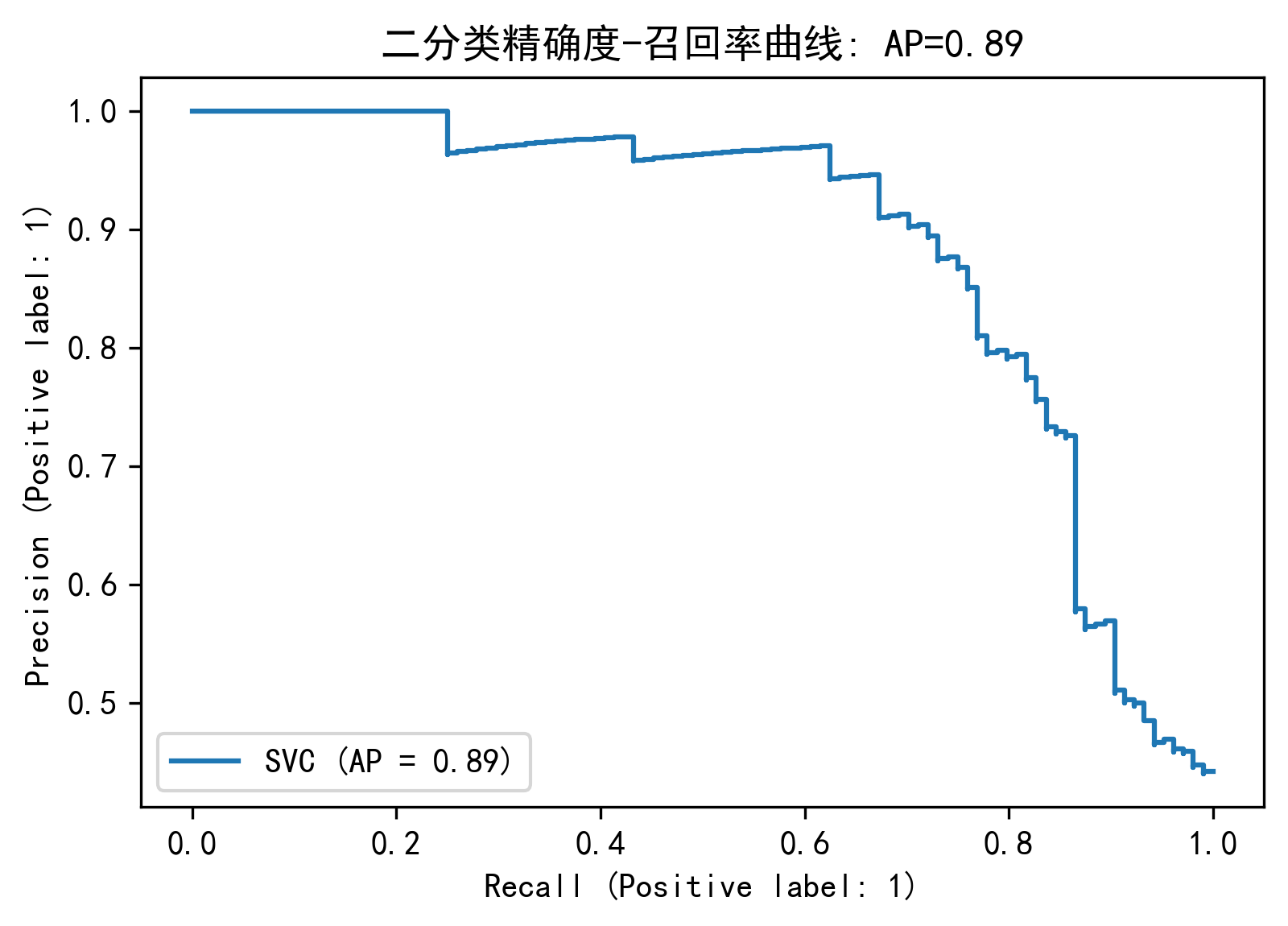
绘制精确度-召回率曲线
1 2 3 4 5 6 7 from sklearn.metrics import average_precision_scorefrom sklearn.metrics import precision_recall_curvefrom sklearn.metrics import plot_precision_recall_curveimport matplotlib.pyplot as pltplt.rcParams['figure.dpi' ] = 300 plt.rcParams['font.sans-serif' ] = ['SimHei' ] plt.rcParams['axes.unicode_minus' ] = False
1 2 3 X_train, X_test, y_train, y_test = train_test_split(X_scaler, y,test_size=0.3 ) y_score=svm_search.best_estimator_.decision_function(X_test) average_precision = average_precision_score(y_test, y_score)
1 print ('平均精确度分数: {0:0.2f}' .format (average_precision))
平均精确度分数: 0.89
1 2 disp = plot_precision_recall_curve(svm_search.best_estimator_, X_test, y_test) disp.ax_.set_title('二分类精确度-召回率曲线: ' 'AP={0:0.2f}' .format (average_precision))
Text(0.5, 1.0, '二分类精确度-召回率曲线: AP=0.89')
自适应提升法
参数
说明
base_estimator object, default = None 建立增强集成的基础估计器。需要支持示例权重,以及适当的classes_和n_classes_属性。如果没有,那么基础估计器是DecisionTreeClassifier(max_depth=1)
n_estimators int, default = 50 终止推进的估计器的最大数目。如果完全拟合,学习过程就会提前停止。
learning_rate float, default = 1 学习率通过learning_rate缩小每个分类器的贡献程度。learning_rate和n_estimators之间存在权衡关系。
algorithm {‘SAMME’, ‘SAMME.R’}, default = ‘SAMME.R’ 若为"SAMME.R"则使用real bossting算法。base_estimator必须支持类概率的计算。若为SAMME,则使用discrete boosting算法。SAMME.R算法的收敛速度通常比SAMME快,通过更少的增强迭代获得更低的测试误差。
random_state int or RandomState, default = None 控制每个base_estimator在每个增强迭代中给定的随机种子。因此,仅在base_estimator引入random_state时使用它。在多个函数调用之间传递可重复输出的整数。见Glossary 。
导入模型
1 from sklearn.ensemble import AdaBoostClassifier
Adaboost模型训练
1 2 from sklearn.model_selection import train_test_splitfrom sklearn.preprocessing import StandardScaler
1 2 3 scaler = StandardScaler() scaler.fit(X) X_scaler = scaler.transform(X)
1 2 3 4 X_train,X_test,Y_train,Y_test=train_test_split(X_scaler,y,test_size=0.3 ) AdaBoost = AdaBoostClassifier(n_estimators=100 ) AdaBoost.fit(X_train, Y_train) print ('准确率:' ,AdaBoost.score(X_test,Y_test))
准确率: 0.8352059925093633
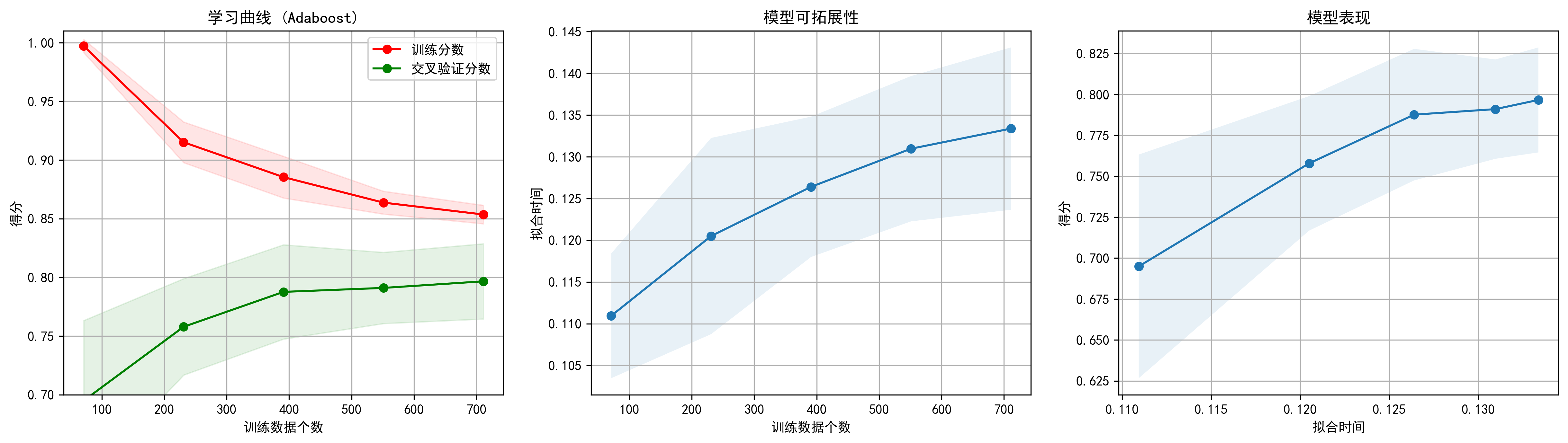
学习曲线
1 2 3 4 5 6 7 8 import numpy as npfrom sklearn.model_selection import learning_curvefrom sklearn.model_selection import ShuffleSplitfrom sklearn.naive_bayes import GaussianNBimport matplotlib.pyplot as pltplt.rcParams['figure.dpi' ] = 300 plt.rcParams['font.sans-serif' ] = ['SimHei' ] plt.rcParams['axes.unicode_minus' ] = False
1 2 3 4 5 6 7 8 9 10 11 12 13 14 15 16 17 18 19 20 21 22 23 24 25 26 27 28 29 30 31 32 33 34 35 36 37 38 39 40 41 42 43 44 45 46 47 48 49 50 51 52 53 54 55 def plot_learning_curve (estimator, title, X, y, axes=None , ylim=None , cv=None ,n_jobs=None , train_sizes=np.linspace(.1 , 1.0 , 5 ): if axes is None : _, axes = plt.subplots(1 , 3 , figsize=(20 , 5 )) axes[0 ].set_title(title) if ylim is not None : axes[0 ].set_ylim(*ylim) axes[0 ].set_xlabel("训练数据个数" ) axes[0 ].set_ylabel("得分" ) train_sizes, train_scores, test_scores, fit_times, _ = \ learning_curve(estimator, X, y, cv=cv, n_jobs=n_jobs, train_sizes=train_sizes, return_times=True ) train_scores_mean = np.mean(train_scores, axis=1 ) train_scores_std = np.std(train_scores, axis=1 ) test_scores_mean = np.mean(test_scores, axis=1 ) test_scores_std = np.std(test_scores, axis=1 ) fit_times_mean = np.mean(fit_times, axis=1 ) fit_times_std = np.std(fit_times, axis=1 ) axes[0 ].grid() axes[0 ].fill_between(train_sizes, train_scores_mean - train_scores_std, train_scores_mean + train_scores_std, alpha=0.1 , color="r" ) axes[0 ].fill_between(train_sizes, test_scores_mean - test_scores_std, test_scores_mean + test_scores_std, alpha=0.1 , color="g" ) axes[0 ].plot(train_sizes, train_scores_mean, 'o-' , color="r" , label="训练分数" ) axes[0 ].plot(train_sizes, test_scores_mean, 'o-' , color="g" , label="交叉验证分数" ) axes[0 ].legend(loc="best" ) axes[1 ].grid() axes[1 ].plot(train_sizes, fit_times_mean, 'o-' ) axes[1 ].fill_between(train_sizes, fit_times_mean - fit_times_std, fit_times_mean + fit_times_std, alpha=0.1 ) axes[1 ].set_xlabel("训练数据个数" ) axes[1 ].set_ylabel("拟合时间" ) axes[1 ].set_title("模型可拓展性" ) axes[2 ].grid() axes[2 ].plot(fit_times_mean, test_scores_mean, 'o-' ) axes[2 ].fill_between(fit_times_mean, test_scores_mean - test_scores_std, test_scores_mean + test_scores_std, alpha=0.1 ) axes[2 ].set_xlabel("拟合时间" ) axes[2 ].set_ylabel("得分" ) axes[2 ].set_title("模型表现" ) return plt
1 2 3 4 5 title = "学习曲线 (Adaboost)" cv = ShuffleSplit(n_splits=10 , test_size=0.2 , random_state=0 ) plot_learning_curve(AdaBoostClassifier(n_estimators=100 ), title, X_scaler, y, ylim=(0.7 , 1.01 ),cv=cv, n_jobs=4 )
无监督学习
数据处理
导入库
1 2 3 4 5 import pandas as pdimport matplotlib.pyplot as pltimport numpy as npfrom sklearn import metricsimport seaborn as sns
读取数据
1 2 df_unsupervised = pd.read_table("agg.txt" , sep='\t' ,engine='python' ) df_unsupervised
x1
x2
y
0
15.55
28.65
2
1
14.90
27.55
2
2
14.45
28.35
2
3
14.15
28.80
2
4
13.75
28.05
2
...
...
...
...
783
7.80
3.35
5
784
8.05
2.75
5
785
8.50
3.25
5
786
8.10
3.55
5
787
8.15
4.00
5
788 rows × 3 columns
1 df_unsupervised.describe()
x1
x2
y
count
788.000000
788.000000
788.000000
mean
19.566815
14.171764
3.770305
std
9.922042
8.089683
1.596305
min
3.350000
1.950000
1.000000
25%
11.150000
7.037500
2.000000
50%
18.225000
11.725000
4.000000
75%
30.700000
21.962500
5.000000
max
36.550000
29.150000
7.000000
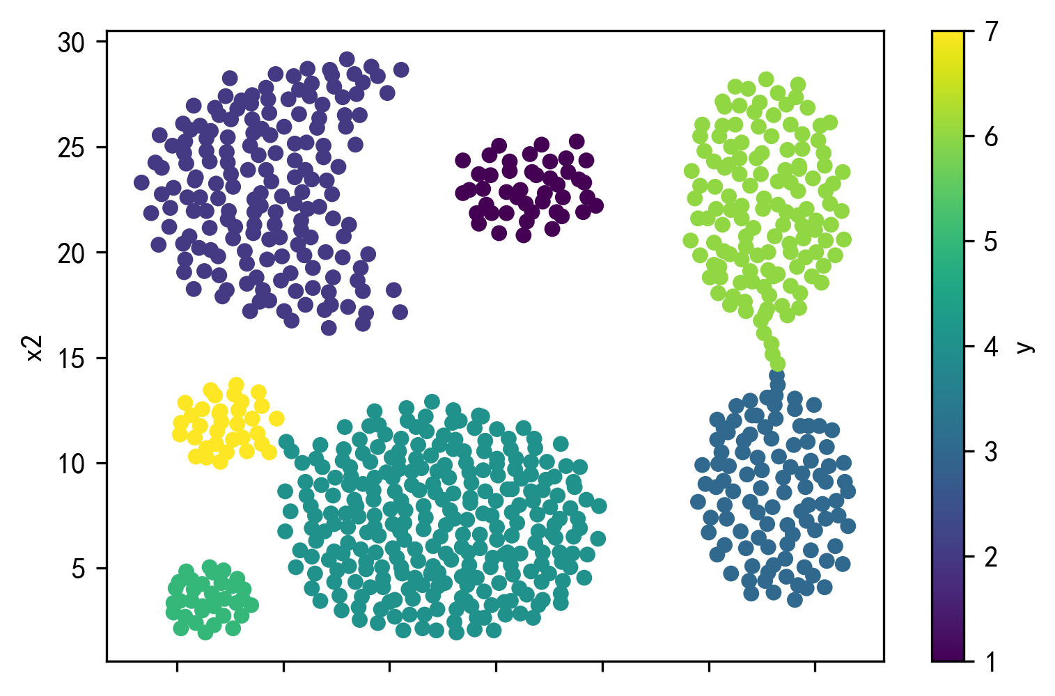
绘制散点图
1 2 df_unsupervised.plot.scatter(x='x1' ,y='x2' ,c='y' ,colormap='viridis' ) plt.show()
1 2 X_unsupervised = df_unsupervised[['x1' , 'x2' ]] Y_unsupervised = df_unsupervised['y' ]
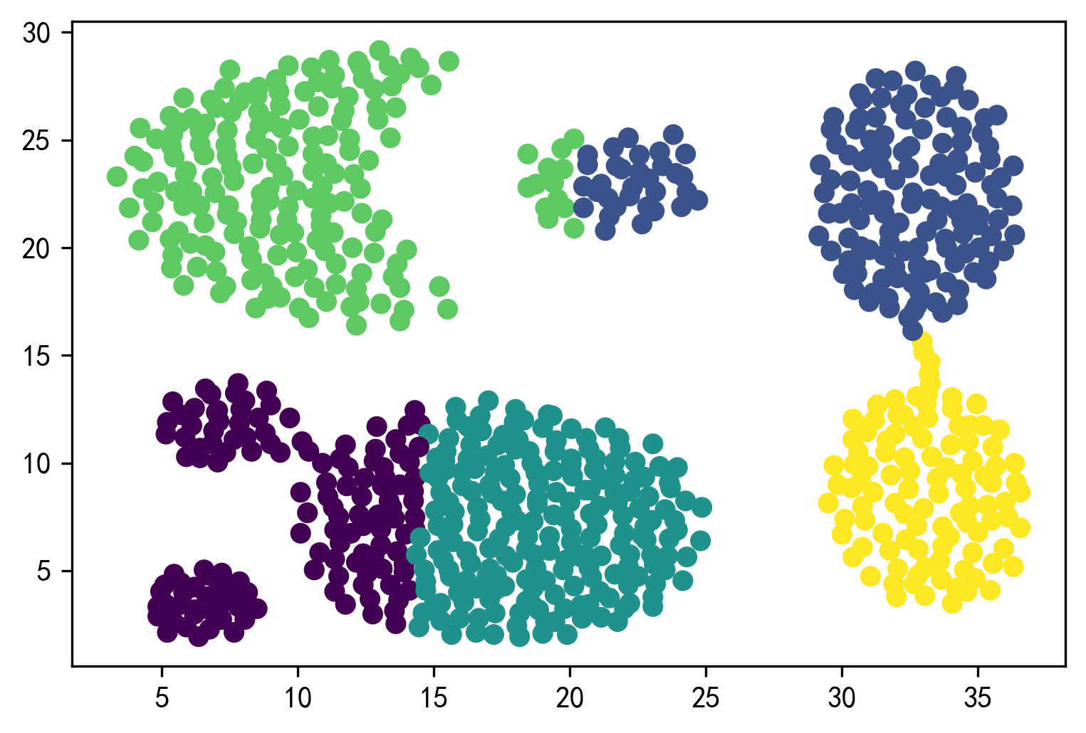
K-means聚类
1 from sklearn.cluster import KMeans
1 2 3 y_unsupervised_pred=KMeans(n_clusters=5 ,random_state=9 ).fit_predict(X_unsupervised) plt.scatter(X_unsupervised['x1' ],X_unsupervised['x2' ],c=y_unsupervised_pred) plt.show()
轮廓分析
1 2 3 4 5 6 7 8 from sklearn.cluster import KMeansfrom sklearn.metrics import silhouette_samples, silhouette_scoreimport matplotlib.pyplot as pltplt.rcParams['figure.dpi' ] = 300 plt.rcParams['font.sans-serif' ] = ['SimHei' ] plt.rcParams['axes.unicode_minus' ] = False import matplotlib.cm as cm
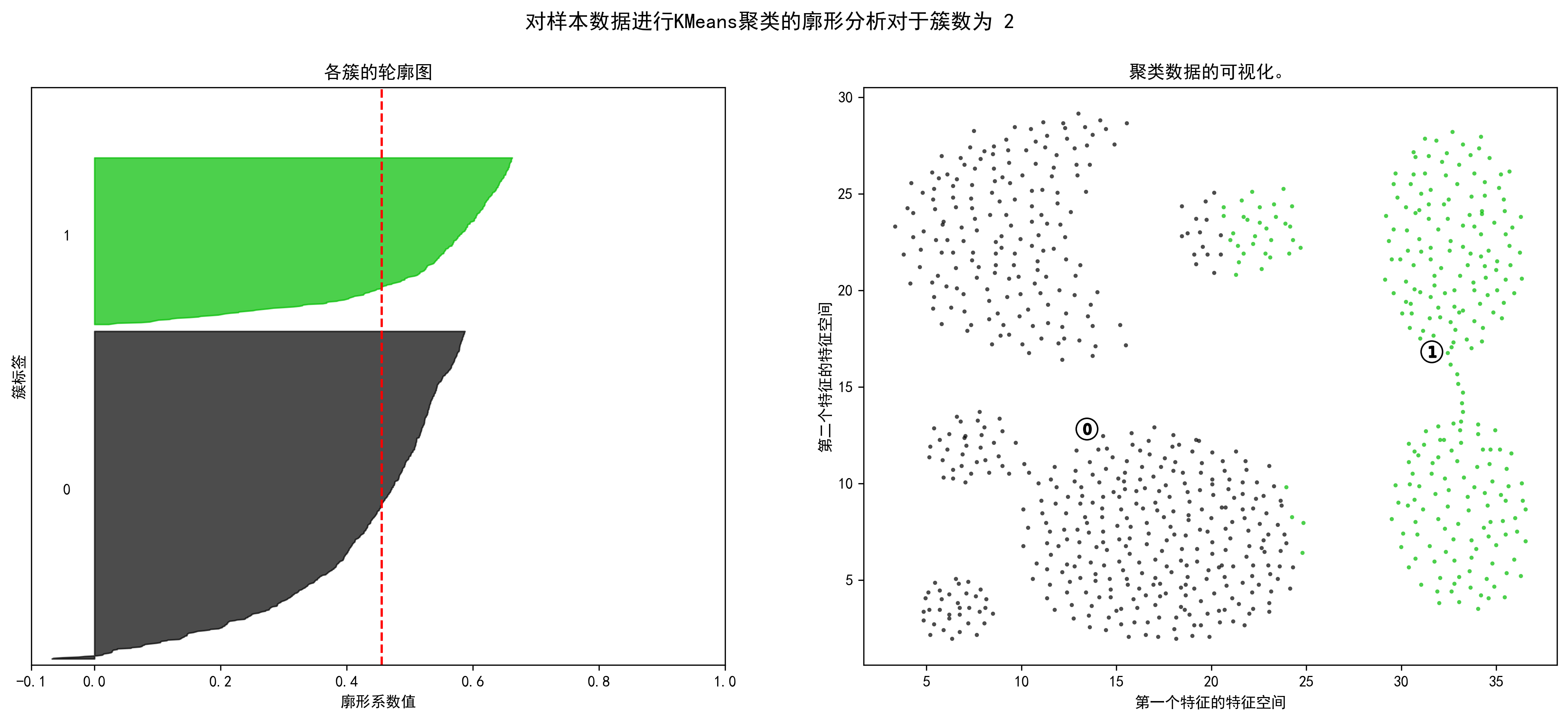
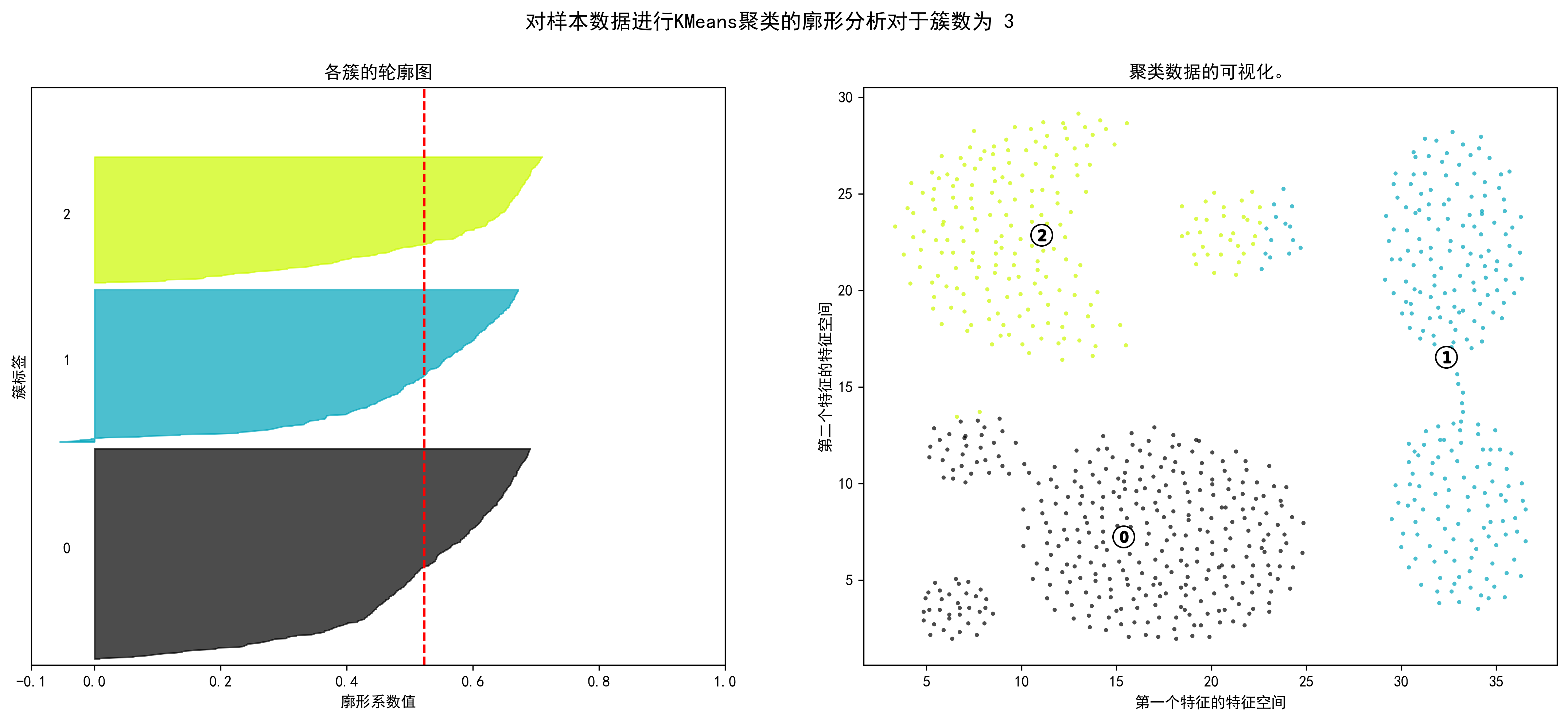
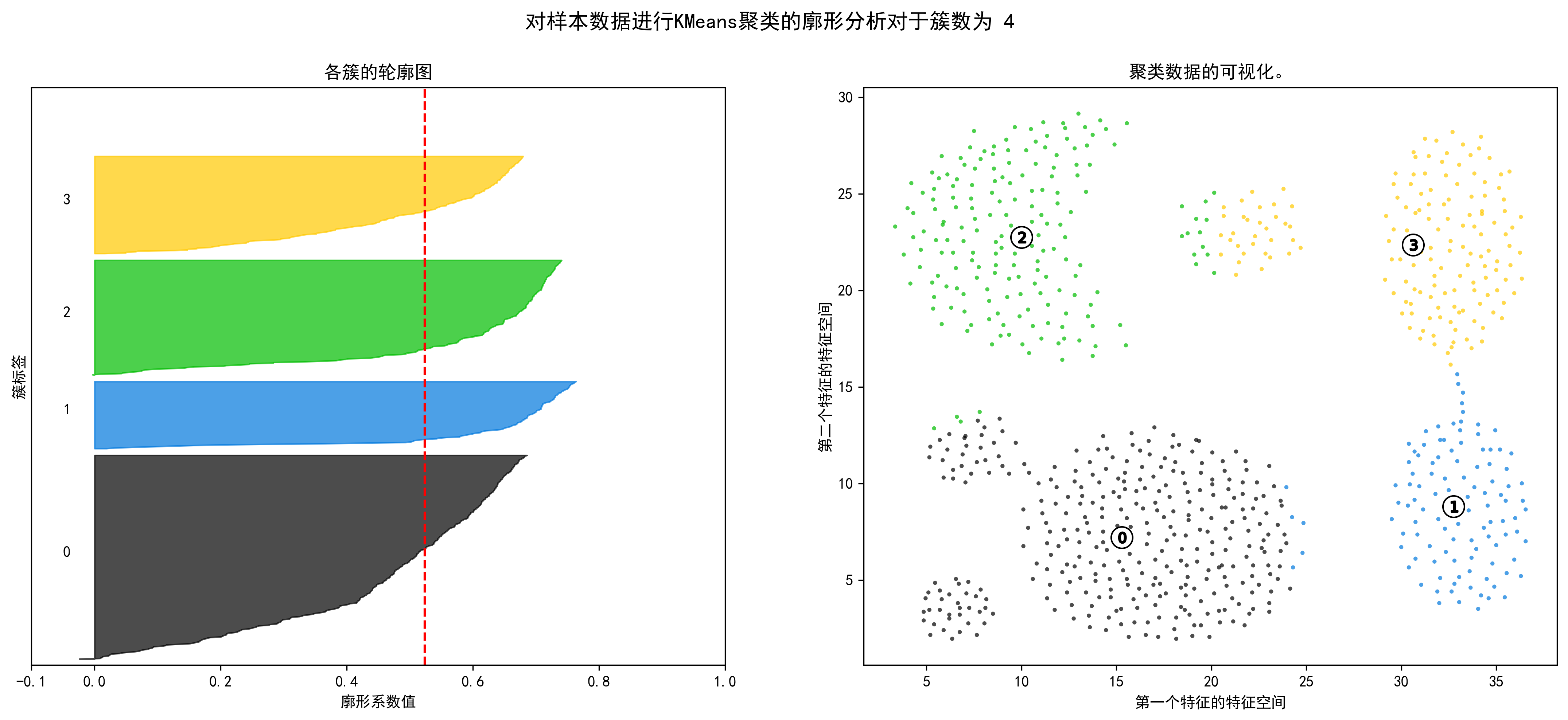
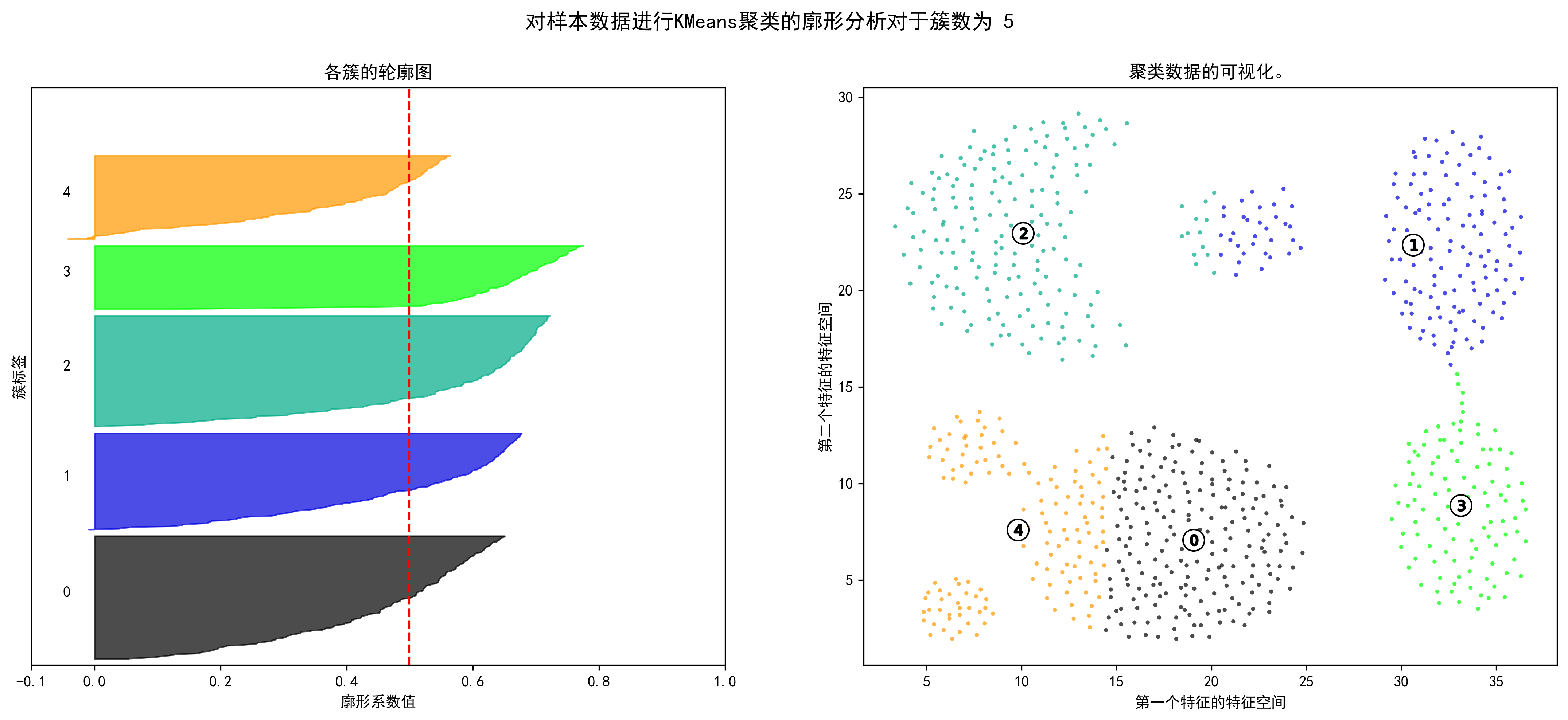
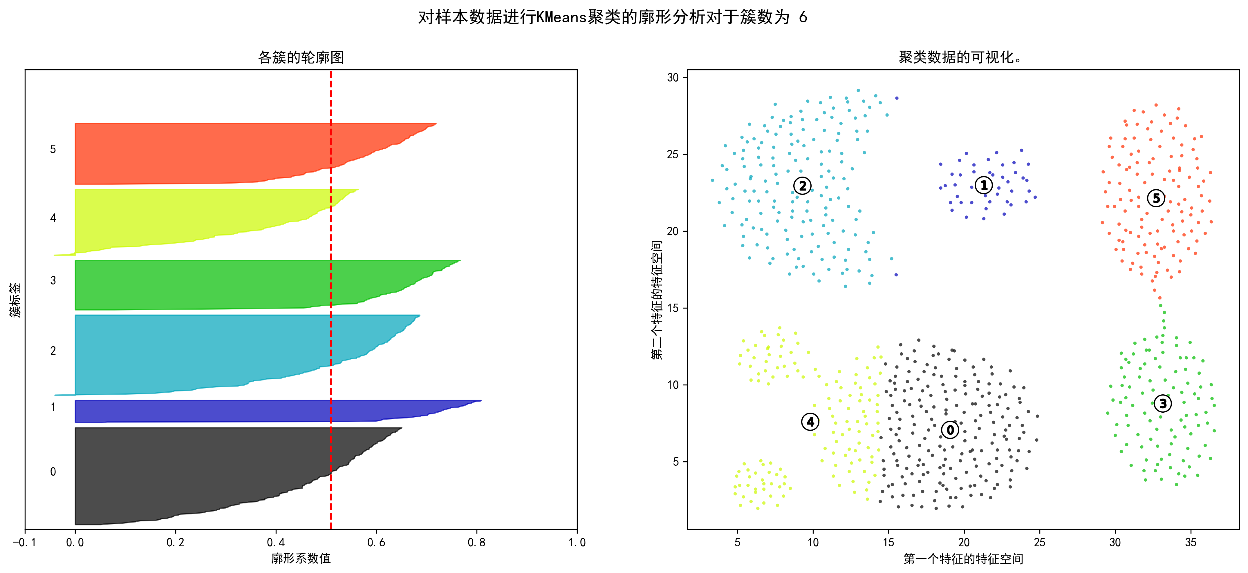
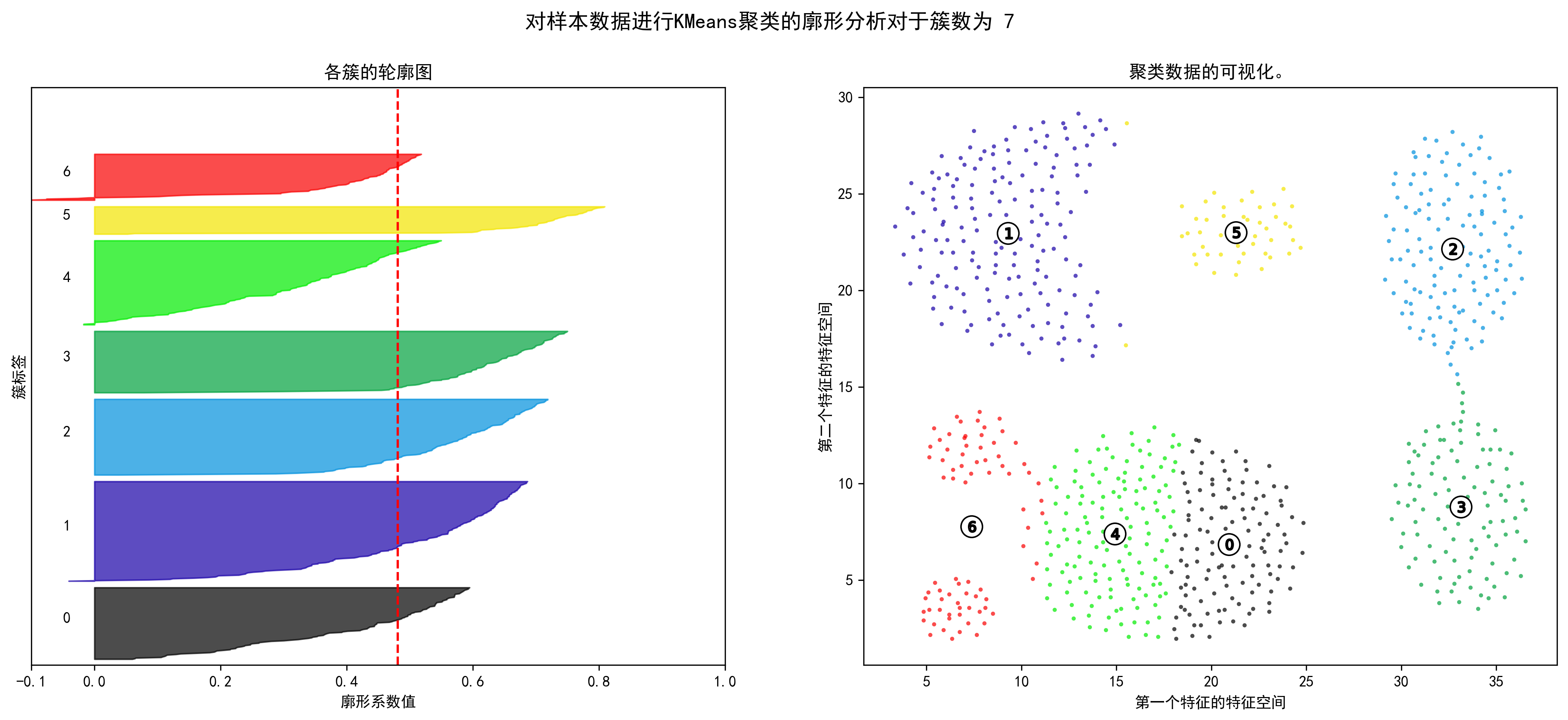
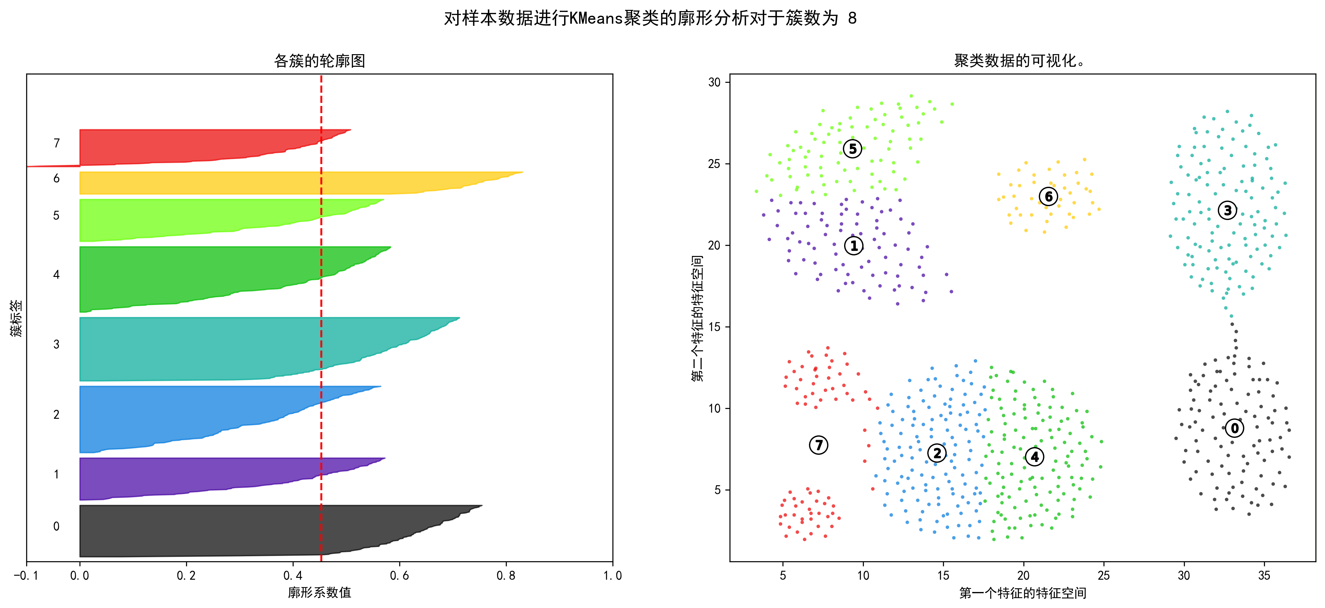
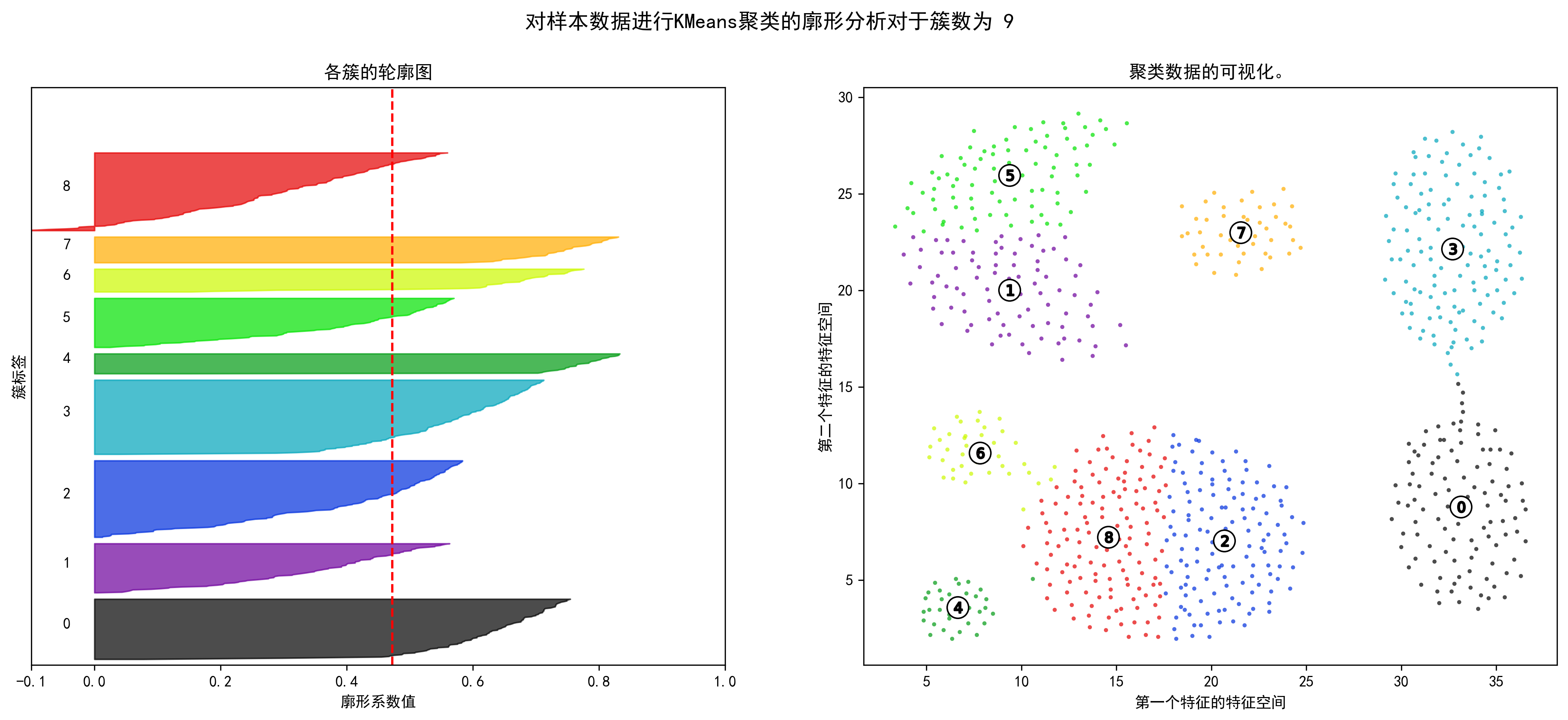
1 2 3 4 5 6 7 8 9 10 11 12 13 14 15 16 17 18 19 20 21 22 23 24 25 26 27 28 29 30 31 32 33 34 35 36 37 38 39 40 41 42 43 44 45 46 47 48 49 50 51 52 53 54 55 56 57 58 59 60 61 62 63 64 65 66 67 68 69 70 71 72 73 74 75 76 77 78 79 80 81 82 83 84 range_n_clusters = np.arange(2 ,10 ) for n_clusters in range_n_clusters: fig, (ax1, ax2) = plt.subplots(1 , 2 ) fig.set_size_inches(18 , 7 ) ax1.set_xlim([-0.1 , 1 ]) ax1.set_ylim([0 , len (X) + (n_clusters + 1 ) * 10 ]) clusterer = KMeans(n_clusters=n_clusters, random_state=10 ) cluster_labels = clusterer.fit_predict(X_unsupervised) silhouette_avg = silhouette_score(X_unsupervised, cluster_labels) print ("对于簇数为" , n_clusters,"平均轮廓得分 :" , silhouette_avg) sample_silhouette_values = silhouette_samples(X_unsupervised, cluster_labels) y_lower = 10 for i in range (n_clusters): ith_cluster_silhouette_values = \ sample_silhouette_values[cluster_labels == i] ith_cluster_silhouette_values.sort() size_cluster_i = ith_cluster_silhouette_values.shape[0 ] y_upper = y_lower + size_cluster_i color = cm.nipy_spectral(float (i) / n_clusters) ax1.fill_betweenx(np.arange(y_lower, y_upper), 0 , ith_cluster_silhouette_values, facecolor=color, edgecolor=color, alpha=0.7 ) ax1.text(-0.05 , y_lower + 0.5 * size_cluster_i, str (i)) y_lower = y_upper + 10 ax1.set_title("各簇的轮廓图" ) ax1.set_xlabel("廓形系数值" ) ax1.set_ylabel("簇标签" ) ax1.axvline(x=silhouette_avg, color="red" , linestyle="--" ) ax1.set_yticks([]) ax1.set_xticks([-0.1 , 0 , 0.2 , 0.4 , 0.6 , 0.8 , 1 ]) colors = cm.nipy_spectral(cluster_labels.astype(float ) / n_clusters) ax2.scatter(X_unsupervised['x1' ], X_unsupervised['x2' ], marker='.' , s=30 , lw=0 , alpha=0.7 ,c=colors, edgecolor='k' ) centers = clusterer.cluster_centers_ ax2.scatter(centers[:, 0 ], centers[:, 1 ], marker='o' ,c="white" , alpha=1 , s=200 , edgecolor='k' ) for i, c in enumerate (centers): ax2.scatter(c[0 ], c[1 ], marker='$%d$' % i, alpha=1 , s=50 , edgecolor='k' ) ax2.set_title("聚类数据的可视化。" ) ax2.set_xlabel("第一个特征的特征空间" ) ax2.set_ylabel("第二个特征的特征空间" ) plt.suptitle(("对样本数据进行KMeans聚类的廓形分析" "对于簇数为 %d" % n_clusters), fontsize=14 , fontweight='bold' ) plt.show()
对于簇数为 2 平均轮廓得分 : 0.4558185732952947
对于簇数为 3 平均轮廓得分 : 0.5233926629564977
对于簇数为 4 平均轮廓得分 : 0.5236026699214911
对于簇数为 5 平均轮廓得分 : 0.4986983771034953
对于簇数为 6 平均轮廓得分 : 0.5092643403975724
对于簇数为 7 平均轮廓得分 : 0.4809820385173227
对于簇数为 8 平均轮廓得分 : 0.45319390110467783
对于簇数为 9 平均轮廓得分 : 0.4725748945562861
DBSCAN聚类
1 from sklearn.cluster import DBSCAN
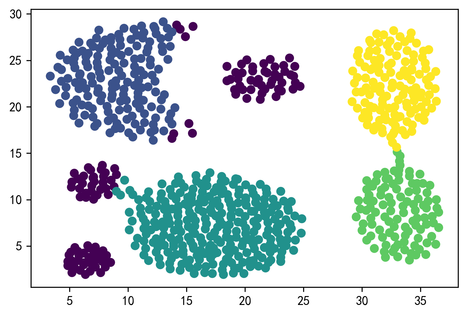
1 2 3 4 5 6 dbs = DBSCAN(eps=3.5 , min_samples=50 ) dbs.fit(X_unsupervised) result = dbs.fit_predict(X_unsupervised) plt.figure() plt.scatter(X_unsupervised['x1' ],X_unsupervised['x2' ], c=result) plt.show()
寻找最优参数
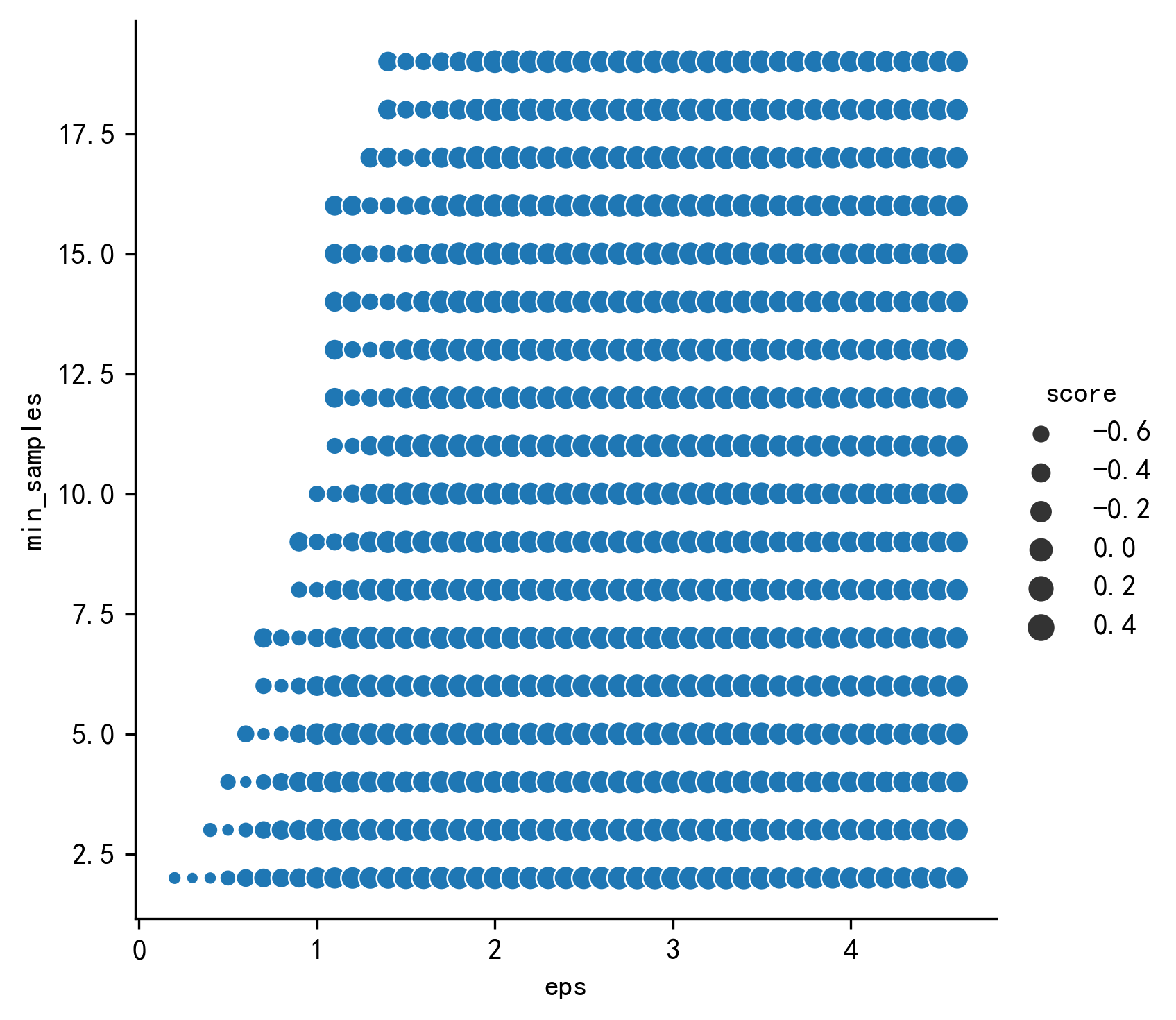
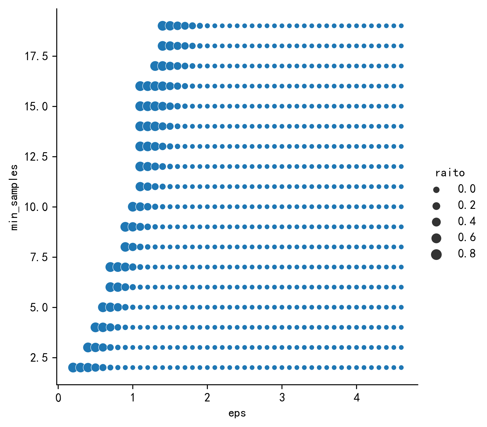
1 2 3 4 5 6 7 8 9 10 11 12 13 14 15 16 17 18 19 20 21 22 23 24 25 26 27 28 29 30 31 rs= [] eps = np.arange(0.2 ,5 ,0.1 ) min_samples=np.arange(2 ,20 ,1 ) best_score=0 best_score_eps=0 best_score_min_samples=0 for i in eps: for j in min_samples: try : db = DBSCAN(eps=i, min_samples=j).fit(X_unsupervised) labels= db.labels_ k=metrics.silhouette_score(X_unsupervised,labels) raito = len (labels[labels[:] == -1 ]) / len (labels) n_clusters_ = len (set (labels)) - (1 if -1 in labels else 0 ) rs.append([i,j,k,raito,n_clusters_]) if k>best_score: best_score=k best_score_eps=i best_score_min_samples=j else : db='' except : db='' rs= pd.DataFrame(rs) rs.columns=['eps' ,'min_samples' ,'score' ,'raito' ,'n_clusters' ] sns.relplot(x="eps" ,y="min_samples" , size='score' ,data=rs) sns.relplot(x="eps" ,y="min_samples" , size='raito' ,data=rs) print ('最优得分' ,best_score,'\n最优得分_eps' ,best_score_eps,'\n最优得分_min_samples' ,best_score_min_samples)
最优得分 0.4868290825347166
最优得分_eps 1.3000000000000003
最优得分_min_samples 7
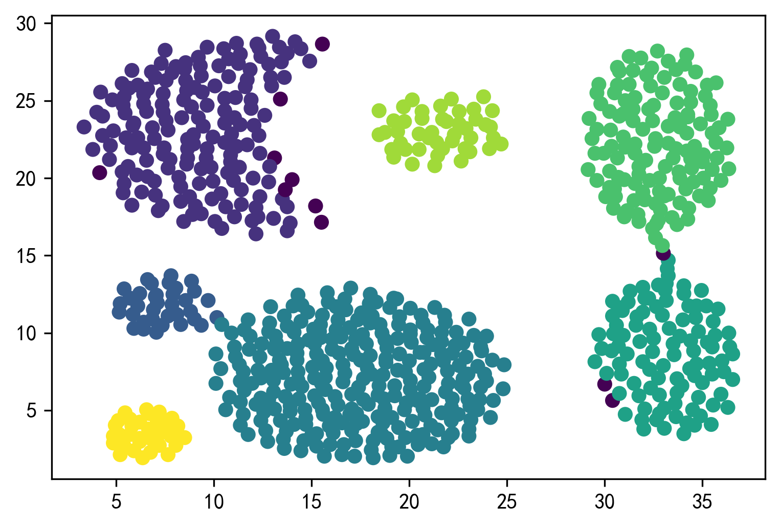
1 2 3 4 5 6 best_model = DBSCAN(eps=best_score_eps, min_samples=best_score_min_samples) best_model.fit(X_unsupervised) result = best_model.fit_predict(X_unsupervised) plt.figure() plt.scatter(X_unsupervised['x1' ],X_unsupervised['x2' ], c=result) plt.show()