前言
虽然这门课叫做心理统计,但是统计的内容几乎不涵盖任何数学公式以及相应的公式推导证明,即使刘红云老师是数学科班出身…据她说,她也是在心理学部摸爬滚打摸索出一条不讲任何数学公式的统计课,适合心理学部宝宝的体质。
多元回归分析
导入包与数据
1 2 3 4 5 6 7 8 9 10 11 12 13 14 15 16 17 library( haven) library( car) library( olsrr) library( psych) library( ggplot2) library( broom) library( ppcor) library( lm.beta) setwd( "/Users/nanxu/研究生课程作业/心理统计/多元回归个人作业数据文件/" ) data <- read_sav( "./3_1.sav" ) names ( data) dim ( data)
标准多元回归
1 2 3 4 5 model <- lm( timedrs ~ phyheal + menheal + stress, data = data) summary( model)
模型拟合情况
1
2
3
Residual standard error: 10.13 on 356 degrees of freedom Multiple R- squared: 0.211 , Adjusted R- squared: 0.2044 F - statistic: 31.74 on 3 and 356 DF, p- value: < 2.2e-16
三个自变量总共可以解释因变量变异的21.1%
标准化回归系数
1 2 3 Standardized Coefficients:: ( Intercept) phyheal menheal stress NA 0.359931424 0.008328805 0.193065466
方差分析
1 2 3 4 5 6 Response: timedrs Df Sum Sq Mean Sq F value Pr( > F ) phyheal 1 8154 8154.1 79.4912 < 2.2e-16 * * * menheal 1 110 110.5 1.0769 0.3000946 stress 1 1502 1501.7 14.6391 0.0001537 * * * Residuals 356 36518 102.6
多重共线性
多重共线性指标
1 2 3 4 5 6 7 8 9 10 11 vif( model) 1 / vif( model) model_std <- lm( timedrs ~ scale( phyheal) + scale( menheal) + scale( stress) , data = data) ols_eigen_cindex( model_std)
1 2 3 4 5 6 7 8 9 10 11 12 > vif( model) phyheal menheal stress 1.361953 1.402107 1.148871 > 1 / vif( model) phyheal menheal stress 0.7342395 0.7132121 0.8704199 > ols_eigen_cindex( model_std) Eigenvalue Condition Index intercept scale( phyheal) scale( menheal) scale( stress) 1 1.7531868 1.000000 0 0.1521228 0.15623913 0.12546381 2 1.0000000 1.324080 1 0.0000000 0.00000000 0.00000000 3 0.7483957 1.530553 0 0.1797878 0.07500899 0.85837173 4 0.4984175 1.875502 0 0.6680894 0.76875189 0.01616446
容忍度TOL大于0.1,且方差膨胀因子VIF小于10,并且条件指数CI为1.875502,三个变量不存在明显的多重共线性问题
残差分析
残差统计量
1 2 3 4 5 describe( fitted( model) ) describe( residuals( model) ) describe( scale( fitted( model) ) ) describe( scale( residuals( model) ) )
根据3SD原则,标准化残差的绝对值大雨3对应的观测值为异常值。
1 2 3 4 5 6 7 8 9 10 11 12 13 14 15 16 > describe( fitted( model) ) vars n mean sd median trimmed mad min max range skew kurtosis se X1 1 360 8.04 5.22 7.37 7.58 4.69 - 0.65 26.98 27.63 0.94 1.03 0.27 > > describe( fitted( model) ) vars n mean sd median trimmed mad min max range skew kurtosis se X1 1 360 8.04 5.22 7.37 7.58 4.69 - 0.65 26.98 27.63 0.94 1.03 0.27 > describe( residuals( model) ) vars n mean sd median trimmed mad min max range skew kurtosis se X1 1 360 0 10.09 - 2.02 - 1.72 4.03 - 15.87 64.22 80.09 3.27 13.56 0.53 > describe( scale( fitted( model) ) ) vars n mean sd median trimmed mad min max range skew kurtosis se X1 1 360 0 1 - 0.13 - 0.09 0.9 - 1.67 3.63 5.3 0.94 1.03 0.05 > describe( scale( residuals( model) ) ) vars n mean sd median trimmed mad min max range skew kurtosis se X1 1 360 0 1 - 0.2 - 0.17 0.4 - 1.57 6.37 7.94 3.27 13.56 0.05
本数据集中存在异常值
Durbin-Watson 检验
1 2 durbinWatsonTest( model)
1 2 3 4 > durbinWatsonTest( model) lag Autocorrelation D- W Statistic p- value 1 0.7842281 0.3184074 0 Alternative hypothesis: rho != 0
Durbin-Watson 检验结果为0.3184074,认为残差可能存在正相关
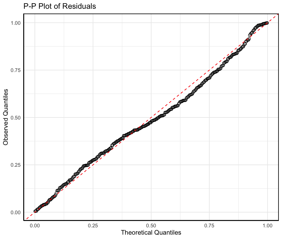
P-P 图 残差累计概率图的散点图
残差的正态性假设指的是每个因变量的预测分数下的残差都呈正态分布。若在P-P图三所有标准化残差都分布在对角线上,则可认为没有违背正态性假设。
1 2 3 4 5 6 7 8 9 10 11 12 13 14 15 16 17 18 19 20 21 22 23 pp_data <- data.frame( Observed = sort( pnorm( scale( residuals( model) ) ) ) , Theoretical = sort( ppoints( length ( scale( residuals( model) ) ) ) ) ) pp_plot <- ggplot( pp_data, aes( x = Theoretical, y = Observed) ) + geom_point( size = 2 , shape = 1 ) + geom_abline( intercept = 0 , slope = 1 , color = "red" , linetype = "dashed" ) + labs( title = "P-P Plot of Residuals" , x = "Theoretical Quantiles" , y = "Observed Quantiles" ) + theme_minimal( ) + theme( panel.border = element_rect( colour = "black" , fill = NA , size = 1 ) , axis.line = element_line( colour = "black" ) ) print( pp_plot)
残差值的点基本上没有分布中对角线上,判定残差不服从正态分布
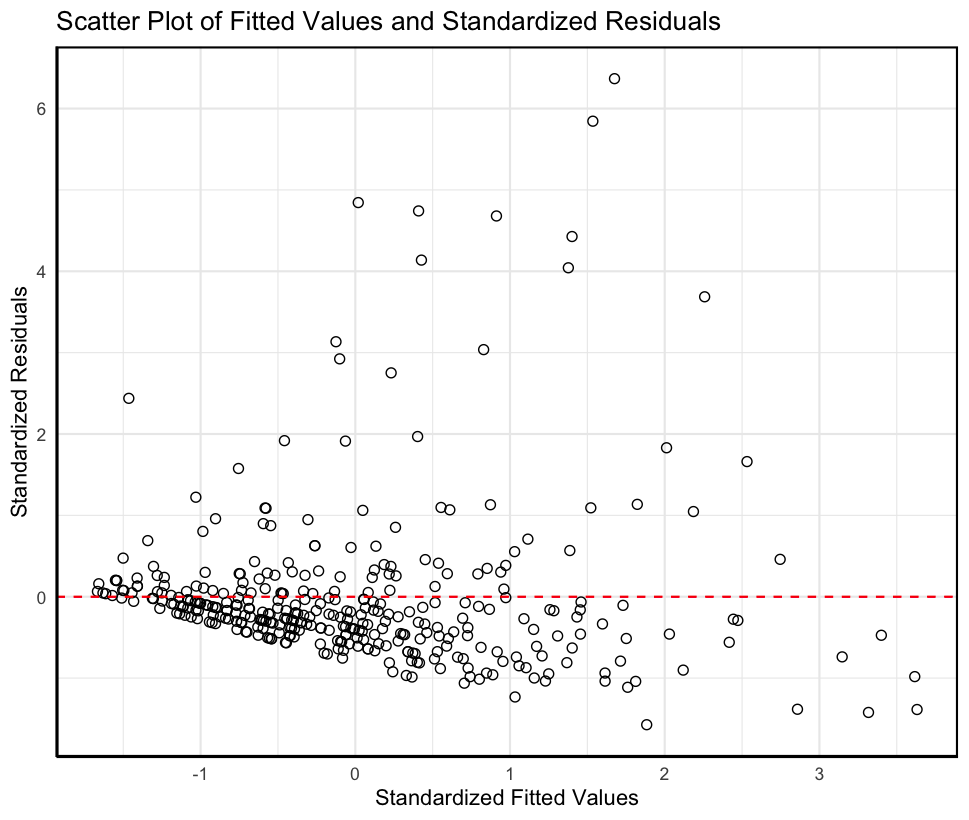
标准化因变量预测值与标准化残差的散点图
1 2 3 4 5 6 7 8 9 10 11 12 13 14 15 16 17 18 19 20 21 22 23 scatter_data <- data.frame( Fitted = scale( fitted( model) ) , Std_Residuals = scale( residuals( model) ) ) scatter_plot <- ggplot( scatter_data, aes( x = Fitted, y = Std_Residuals) ) + geom_point( size = 2 , shape = 1 ) + geom_hline( yintercept = 0 , color = "red" , linetype = "dashed" ) + labs( title = "Scatter Plot of Fitted Values and Standardized Residuals" , x = "Standardized Fitted Values" , y = "Standardized Residuals" ) + theme_minimal( ) + theme( panel.border = element_rect( colour = "black" , fill = NA , size = 1 ) , axis.line = element_line( colour = "black" ) ) print( scatter_plot)
图中各点没有随机分布在一条穿过零点的水平直线的两侧,表明残差的分布不满足正态及残差方差齐次性假设
因变量对数转换的多元回归分析
1 2 3 4 5 6 model_log <- lm( logtimedrs ~ phyheal + menheal + stress, data = data) summary( model_log) lm.beta( model_log) anova( model_log)
1 2 3 4 5 6 7 8 9 10 11 12 13 14 Residual standard error: 0.7752 on 356 degrees of freedom Multiple R- squared: 0.3471 , Adjusted R- squared: 0.3416 F - statistic: 63.08 on 3 and 356 DF, p- value: < 2.2e-16 Standardized Coefficients:: ( Intercept) phyheal menheal stress NA 0.49088568 0.03005799 0.18537313 Response: logtimedrs Df Sum Sq Mean Sq F value Pr( > F ) phyheal 1 102.505 102.505 170.5668 < 2.2e-16 * * * menheal 1 1.429 1.429 2.3773 0.124 stress 1 9.801 9.801 16.3087 6.594e-05 * * * Residuals 356 213.945 0.601
可见因变量对数转换后的回归方程R2 有所升高,回归方程更加显著
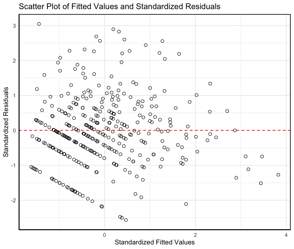
1 2 3 4 5 6 7 8 9 10 11 12 13 14 15 16 17 18 19 20 21 22 23 24 25 26 27 28 29 30 31 32 33 34 35 36 37 38 39 40 41 42 43 pp_data <- data.frame( Observed = sort( pnorm( scale( residuals( model_log) ) ) ) , Theoretical = sort( ppoints( length ( scale( residuals( model_log) ) ) ) ) ) pp_plot <- ggplot( pp_data, aes( x = Theoretical, y = Observed) ) + geom_point( size = 2 , shape = 1 ) + geom_abline( intercept = 0 , slope = 1 , color = "red" , linetype = "dashed" ) + labs( title = "P-P Plot of Residuals" , x = "Theoretical Quantiles" , y = "Observed Quantiles" ) + theme_minimal( ) + theme( panel.border = element_rect( colour = "black" , fill = NA , size = 1 ) , axis.line = element_line( colour = "black" ) ) print( pp_plot) scatter_data <- data.frame( Fitted = scale( fitted( model_log) ) , Std_Residuals = scale( residuals( model_log) ) ) scatter_plot <- ggplot( scatter_data, aes( x = Fitted, y = Std_Residuals) ) + geom_point( size = 2 , shape = 1 ) + geom_hline( yintercept = 0 , color = "red" , linetype = "dashed" ) + labs( title = "Scatter Plot of Fitted Values and Standardized Residuals" , x = "Standardized Fitted Values" , y = "Standardized Residuals" ) + theme_minimal( ) + theme( panel.border = element_rect( colour = "black" , fill = NA , size = 1 ) , axis.line = element_line( colour = "black" ) ) print( scatter_plot)
因变量对数转换后的回归方程基本满足正态性假设以及残差方差齐次性假设
提取回归系数估计和95%置信区间
1 2 tidy( model_log, conf.int = TRUE , conf.level = 0.95 )
1 2 3 4 5 6 7 8 > tidy( model_log, conf.int = TRUE , conf.level = 0.95 ) term estimate std.error statistic p.value conf.low conf.high < chr> < dbl> < dbl> < dbl> < dbl> < dbl> < dbl> 1 ( Intercept) 0.402 0.105 3.83 1.50 e- 4 0.195 0.608 2 phyheal 0.204 0.0208 9.82 2.63e-20 0.163 0.245 3 menheal 0.00681 0.0115 0.593 5.54 e- 1 - 0.0158 0.0294 4 stress 0.00132 0.000327 4.04 6.59 e- 5 0.000677 0.00196
相关系数
零相关系数
1 2 corr.test( data[ c ( "logtimedrs" , "phyheal" , "menheal" , "stress" ) ] )
1 2 logtimedrs phyheal menheal stress logtimedrs 1.00 0.56 0.34 0.34
偏相关系数
1 2 pcor( data[ c ( "logtimedrs" , "phyheal" , "menheal" , "stress" ) ] )
1 2 logtimedrs phyheal menheal stress logtimedrs 1.00000000 0.46174569 0.03139996 0.20929484
半偏相关系数
1 2 spcor( data[ c ( "logtimedrs" , "phyheal" , "menheal" , "stress" ) ] )
1 2 logtimedrs phyheal menheal stress logtimedrs 1.00000000 0.42062902 0.02538454 0.17294627
序列回归
1 2 3 4 5 6 7 8 9 10 11 12 model1 <- lm( logtimedrs ~ phyheal, data = data) summary( model1, standardized= TRUE ) lm.beta( model1) corr.test( data[ c ( "logtimedrs" , "phyheal" ) ] ) pcor( data[ c ( "logtimedrs" , "phyheal" ) ] ) spcor( data[ c ( "logtimedrs" , "phyheal" ) ] )
1 2 3 4 5 6 7 8 9 10 11 12 13 14 15 16 17 18 19 20 21 22 23 24 25 26 27 28 29 30 > summary( model1, standardized= TRUE ) Coefficients: Estimate Std. Error t value Pr( > | t| ) ( Intercept) 0.57627 0.09877 5.834 1.21e-08 * * * phyheal 0.23250 0.01821 12.766 < 2e-16 * * * - - - Residual standard error: 0.7931 on 358 degrees of freedom Multiple R- squared: 0.3128 , Adjusted R- squared: 0.3109 F - statistic: 163 on 1 and 358 DF, p- value: < 2.2e-16 > lm.beta( model1) Standardized Coefficients:: ( Intercept) phyheal NA 0.5593045 > > corr.test( data[ c ( "logtimedrs" , "phyheal" ) ] ) Correlation matrix logtimedrs phyheal logtimedrs 1.00 0.56 > > pcor( data[ c ( "logtimedrs" , "phyheal" ) ] ) logtimedrs phyheal logtimedrs 1.0000000 0.5593045 > > spcor( data[ c ( "logtimedrs" , "phyheal" ) ] ) logtimedrs phyheal logtimedrs 1.0000000 0.5593045
身体健康症状phyheal的零阶相关系数、偏相关系数与半偏相关系数相等
1 2 3 4 5 6 7 8 9 10 model2 <- lm( logtimedrs ~ phyheal + stress, data = data) lm.beta( model2) summary( model2, standardized= TRUE ) corr.test( data[ c ( "logtimedrs" , "phyheal" , "stress" ) ] ) pcor( data[ c ( "logtimedrs" , "phyheal" , "stress" ) ] ) spcor( data[ c ( "logtimedrs" , "phyheal" , "stress" ) ] )
1 2 3 4 5 6 7 8 9 10 11 12 13 14 15 16 17 18 19 20 21 22 23 24 25 26 27 28 29 30 > summary( model2, standardized= TRUE ) Coefficients: Estimate Std. Error t value Pr( > | t| ) ( Intercept) 0.4074062 0.1041975 3.910 0.00011 * * * phyheal 0.2095523 0.0185741 11.282 < 2e-16 * * * stress 0.0013633 0.0003181 4.286 2.35e-05 * * * - - - Residual standard error: 0.7745 on 357 degrees of freedom Multiple R- squared: 0.3464 , Adjusted R- squared: 0.3428 F - statistic: 94.62 on 2 and 357 DF, p- value: < 2.2e-16 > lm.beta( model2) Standardized Coefficients:: ( Intercept) phyheal stress NA 0.5041089 0.1915007 > > corr.test( data[ c ( "logtimedrs" , "phyheal" , "stress" ) ] ) logtimedrs phyheal stress logtimedrs 1.00 0.56 0.34 > > pcor( data[ c ( "logtimedrs" , "phyheal" , "stress" ) ] ) logtimedrs phyheal stress logtimedrs 1.0000000 0.5126673 0.2212089 > > spcor( data[ c ( "logtimedrs" , "phyheal" , "stress" ) ] ) logtimedrs phyheal stress logtimedrs 1.0000000 0.4827156 0.1833739
1 2 3 model3 <- lm( logtimedrs ~ phyheal + stress + menheal, data = data) summary( model3, standardized= TRUE )
1 2 3 4 5 6 7 8 9 10 11 12 13 14 15 16 17 18 19 20 21 22 23 24 25 26 27 28 29 30 31 > summary( model3, standardized= TRUE ) Coefficients: Estimate Std. Error t value Pr( > | t| ) ( Intercept) 0.4015263 0.1047630 3.833 0.00015 * * * phyheal 0.2040556 0.0207754 9.822 < 2e-16 * * * stress 0.0013197 0.0003268 4.038 6.59e-05 * * * menheal 0.0068070 0.0114839 0.593 0.55373 - - - Residual standard error: 0.7752 on 356 degrees of freedom Multiple R- squared: 0.3471 , Adjusted R- squared: 0.3416 F - statistic: 63.08 on 3 and 356 DF, p- value: < 2.2e-16 > lm.beta( model3) Standardized Coefficients:: ( Intercept) phyheal stress menheal NA 0.49088568 0.18537313 0.03005799 > > corr.test( data[ c ( "logtimedrs" , "phyheal" , "menheal" , "stress" ) ] ) logtimedrs phyheal menheal stress logtimedrs 1.00 0.56 0.34 0.34 > > pcor( data[ c ( "logtimedrs" , "phyheal" , "menheal" , "stress" ) ] ) logtimedrs phyheal menheal stress logtimedrs 1.00000000 0.46174569 0.03139996 0.20929484 > > spcor( data[ c ( "logtimedrs" , "phyheal" , "menheal" , "stress" ) ] ) logtimedrs phyheal menheal stress logtimedrs 1.00000000 0.42062902 0.02538454 0.17294627
可以看出,模型三加入menheal并没有带来R2 显著的变化,表明新加入的变量对预测因变量没有显著的贡献。并且心理健康症状menheal的标准化系数为0.03005799,不能显著预测看病次数。偏相关系数为0.03139996且半偏相关系数为0.02538454,与零阶相关系数0.34相差较大,表明menheal不能预测看病次数。
1 2 3 4 5 6 7 8 9 10 > anova( model1, model2, model3) Analysis of Variance Table Model 1 : logtimedrs ~ phyheal Model 2 : logtimedrs ~ phyheal + stress Model 3 : logtimedrs ~ phyheal + stress + menheal Res.Df RSS Df Sum of Sq F Pr( > F ) 1 358 225.18 2 357 214.16 1 11.0186 18.3347 2.386e-05 * * * 3 356 213.94 1 0.2111 0.3513 0.5537
EFA
导入包与数据
1 2 3 4 5 6 7 8 9 10 11 12 library( haven) library( psych) library( GPArotation) setwd( "/Users/nanxu/研究生课程作业/心理统计/课件数据/7第七章 探索性因素分析/" ) data <- read_sav( "./7_2.sav" ) names ( data) dim ( data)
数据预处理
1 2 3 4 5 6 7 8 9 10 11 12 13 analysis_data <- data[ , 1 : 32 ] analysis_data[ analysis_data == - 1 ] <- NA colSums( is.na ( analysis_data) ) describe( analysis_data)
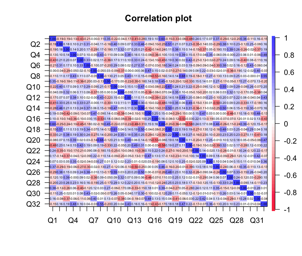
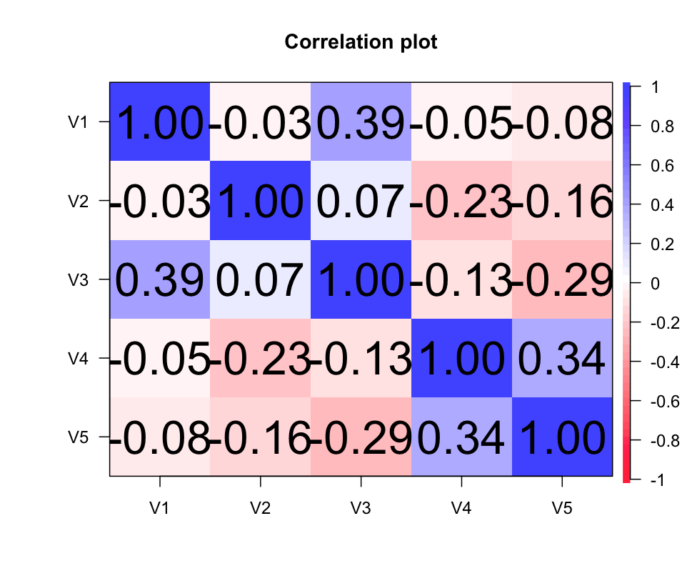
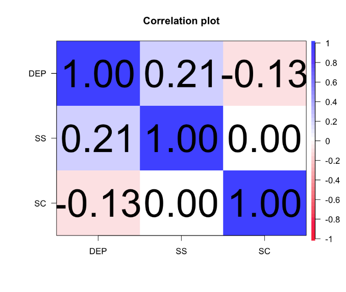
1 2 3 4 5 6 7 8 9 cor_matrix <- cor( analysis_data, use= "complete.obs" ) cor.plot( cor_matrix) KMO( cor_matrix) cortest.bartlett( cor_matrix, n = nrow( analysis_data) )
1 2 3 4 5 6 7 8 9 10 11 12 13 14 15 16 17 18 19 > KMO( cor_matrix) Kaiser- Meyer- Olkin factor adequacy Call: KMO( r = cor_matrix) Overall MSA = 0.86 MSA for each item = Q1 Q2 Q3 Q4 Q5 Q6 Q7 Q8 Q9 Q10 Q11 Q12 Q13 Q14 Q15 Q16 Q17 Q18 Q19 Q20 Q21 Q22 Q23 Q24 Q25 Q26 Q27 0.91 0.90 0.90 0.87 0.87 0.79 0.79 0.82 0.91 0.85 0.86 0.88 0.89 0.90 0.82 0.86 0.88 0.83 0.91 0.82 0.89 0.85 0.81 0.82 0.83 0.88 0.83 Q28 Q29 Q30 Q31 Q32 0.87 0.87 0.76 0.82 0.90 > cortest.bartlett( cor_matrix, n = nrow( analysis_data) ) $ chisq[ 1 ] 4504.689 $ p.value[ 1 ] 0 $ df[ 1 ] 496
KMO的值为0.86大于0.5接近1;Bartlett球形检验结果是显著的;反映像相关矩阵MSA都大于0.5,适合做因素分析。
确定因子数目
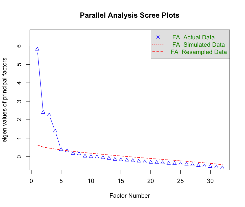
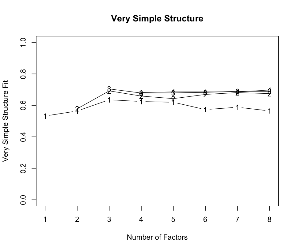
1 2 3 fa.parallel( analysis_data, fa= "fa" , n.iter= 500 ) vss( analysis_data, rotate = "promax" , fm = "pa" )
可以看出,碎石图的拐点位于5个因素的位置
因素数固定为7的探索性因素分析
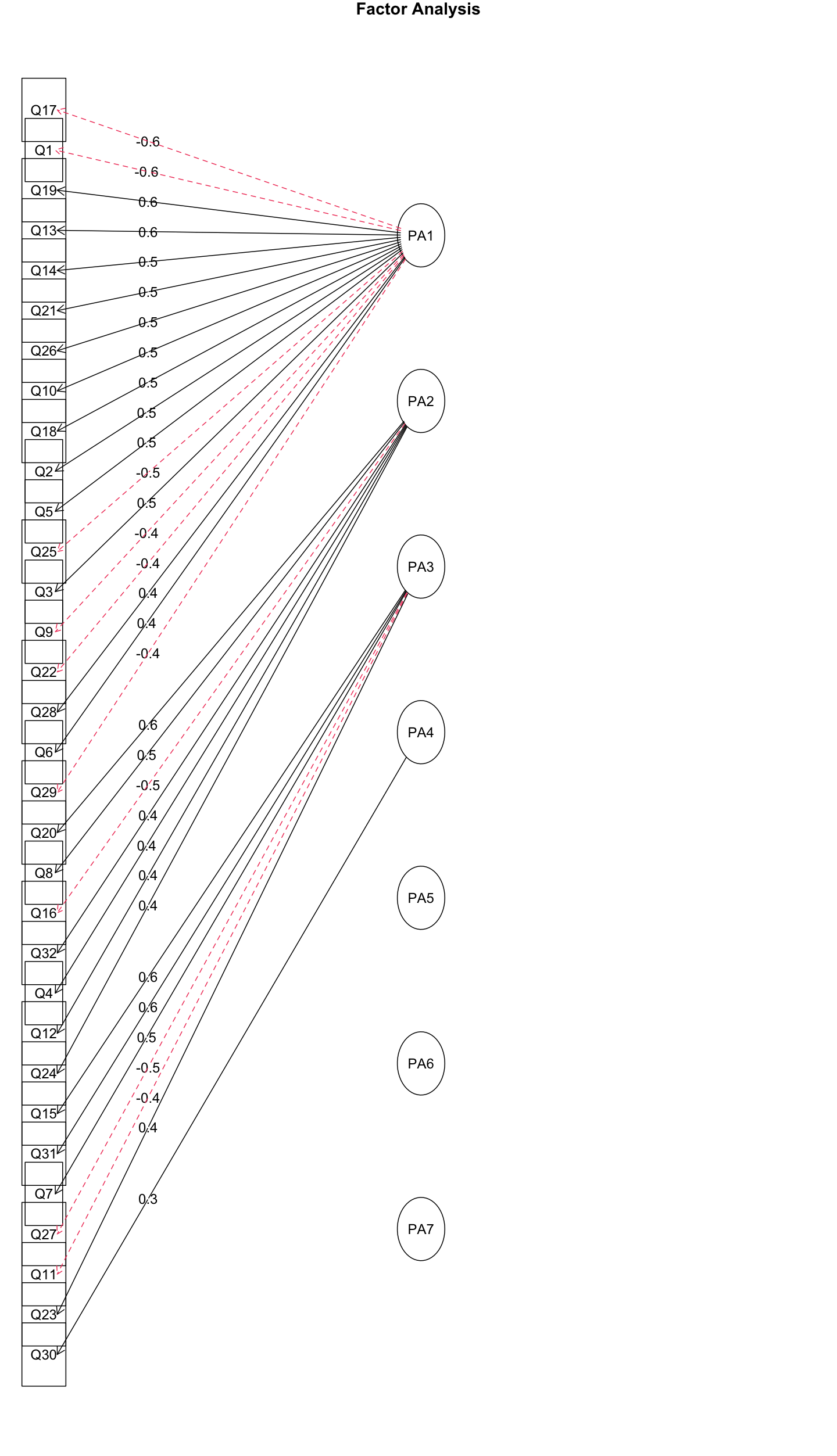
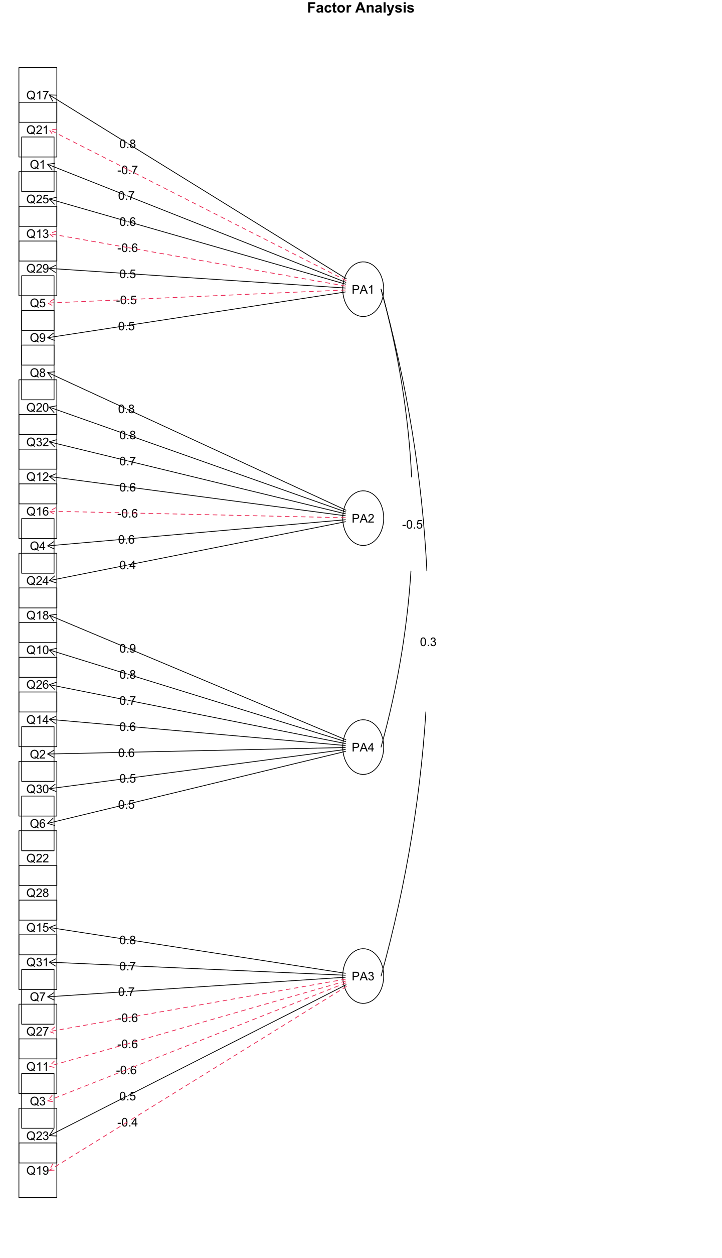
1 2 3 4 5 6 7 8 9 10 11 12 13 efa_7_pa <- fa( analysis_data, nfactors= 7 , rotate= "none" , fm= "pa" ) efa_7_pa$ Vaccounted efa_7_pa$ communality efa_7_pa$ loadings print( efa_7_pa$ loadings, cutoff= 0.3 ) plot( efa_7_pa) fa.diagram( efa_7_pa)
1 2 3 4 5 6 7 8 9 10 11 12 13 14 15 16 17 18 19 20 21 22 23 24 25 26 27 28 29 30 31 32 33 34 35 36 37 38 39 40 41 42 43 44 45 46 47 48 49 50 > efa_7_pa$ Vaccounted PA1 PA2 PA3 PA4 PA5 PA6 PA7 SS loadings 6.0813377 2.73434132 2.61094942 1.65202904 0.64506901 0.56737623 0.45388757 Proportion Var 0.1900418 0.08544817 0.08159217 0.05162591 0.02015841 0.01773051 0.01418399 Cumulative Var 0.1900418 0.27548997 0.35708214 0.40870804 0.42886645 0.44659696 0.46078095 Proportion Explained 0.4124342 0.18544206 0.17707366 0.11204002 0.04374835 0.03847925 0.03078249 Cumulative Proportion 0.4124342 0.59787622 0.77494988 0.88698990 0.93073825 0.96921751 1.00000000 > efa_7_pa$ communality Q1 Q2 Q3 Q4 Q5 Q6 Q7 Q8 Q9 Q10 Q11 Q12 Q13 0.5301886 0.4358322 0.4134696 0.4153618 0.3550281 0.3194059 0.3771826 0.6217469 0.2791207 0.5942034 0.3818267 0.4474353 0.5873971 Q14 Q15 Q16 Q17 Q18 Q19 Q20 Q21 Q22 Q23 Q24 Q25 Q26 0.4835861 0.6512268 0.4792159 0.6518687 0.6188608 0.4615502 0.5965053 0.5176691 0.4549469 0.3967925 0.2961682 0.4942008 0.4989878 Q27 Q28 Q29 Q30 Q31 Q32 0.4268663 0.2830110 0.4525763 0.2163821 0.5086944 0.4976820 > print( efa_7_pa$ loadings, cutoff= 0.3 ) Loadings: PA1 PA2 PA3 PA4 PA5 PA6 PA7 Q1 - 0.579 Q2 0.508 Q3 0.467 - 0.398 Q4 0.332 0.413 Q5 0.482 Q6 0.414 Q7 - 0.301 0.460 Q8 0.422 0.527 0.359 Q9 - 0.443 Q10 0.527 0.460 Q11 - 0.443 Q12 0.353 0.389 0.302 Q13 0.556 0.318 Q14 0.547 Q15 - 0.367 - 0.304 0.603 Q16 - 0.327 - 0.514 Q17 - 0.642 0.368 Q18 0.518 0.507 Q19 0.558 Q20 0.392 0.588 Q21 0.536 - 0.312 - 0.311 Q22 - 0.437 0.378 Q23 - 0.362 0.373 Q24 0.354 Q25 - 0.471 0.350 Q26 0.534 0.303 Q27 - 0.451 Q28 0.419 Q29 - 0.360 0.317 Q30 0.306 Q31 - 0.352 0.571 Q32 0.437 0.444
可以看出,总体方差解释率为46.078095%
并且在第7个因素上,没有任何一个变量的因素载荷绝对值大于0.3,且在第5、6个因素上,都各只有一个变量的因素载荷绝对值大于0.3
因素数固定为5的探索性因素分析
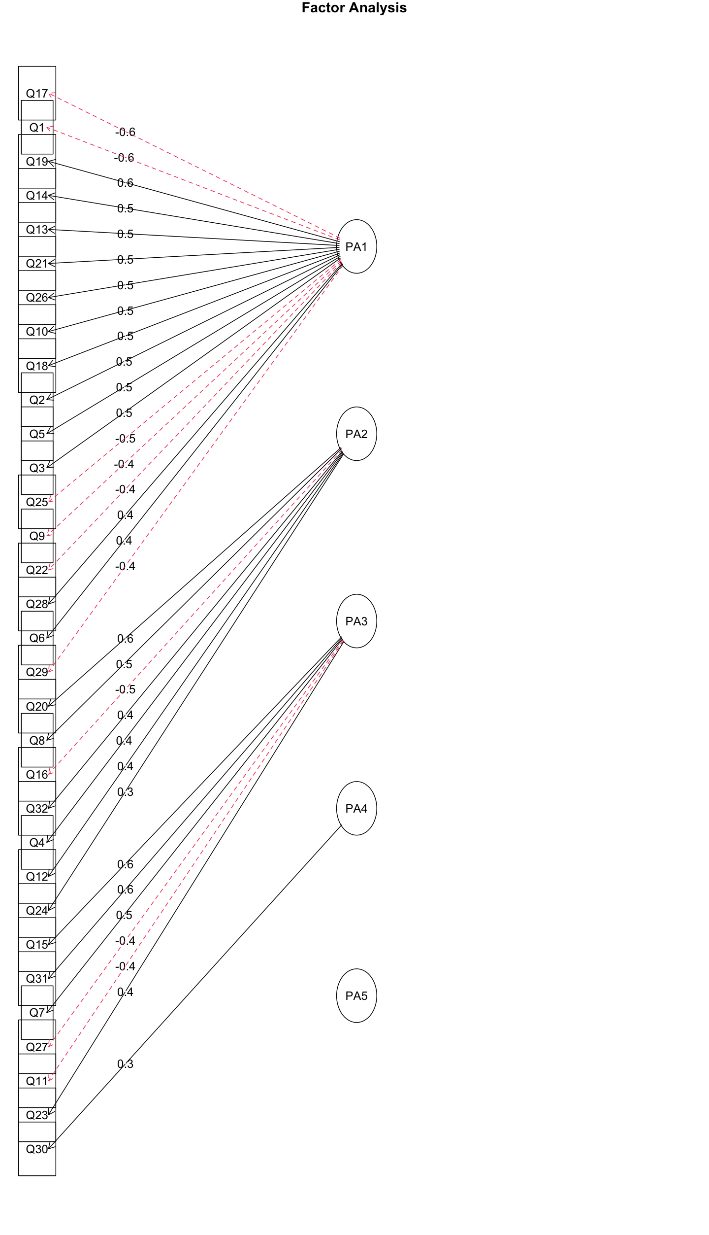
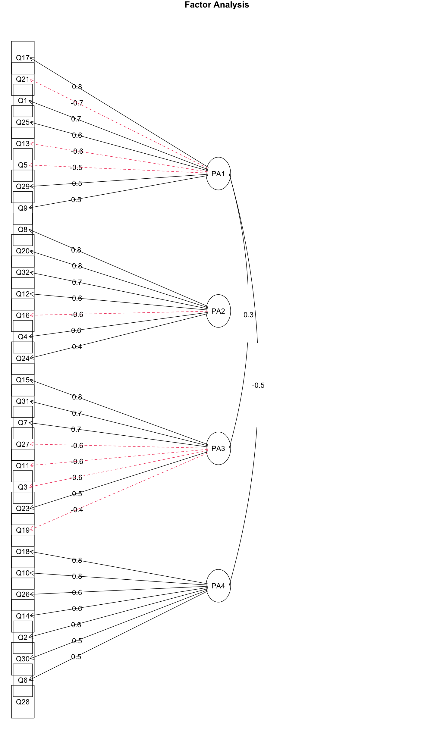
1 2 3 4 5 6 7 8 9 10 11 12 13 efa_5_pa <- fa( analysis_data, nfactors= 5 , rotate= "none" , fm= "pa" ) efa_5_pa$ Vaccounted efa_5_pa$ communality efa_5_pa$ loadings print( efa_5_pa$ loadings, cutoff= 0.3 ) plot( efa_5_pa) fa.diagram( efa_5_pa)
1 2 3 4 5 6 7 8 9 10 11 12 13 14 15 16 17 18 19 20 21 22 23 24 25 26 27 28 29 30 31 32 33 34 35 36 37 38 39 40 41 42 43 44 45 46 47 48 49 50 51 > efa_5_pa$ Vaccounted PA1 PA2 PA3 PA4 PA5 SS loadings 6.0447895 2.70811626 2.58239077 1.62184075 0.59269854 Proportion Var 0.1888997 0.08462863 0.08069971 0.05068252 0.01852183 Cumulative Var 0.1888997 0.27352830 0.35422802 0.40491054 0.42343237 Proportion Explained 0.4461153 0.19986340 0.19058465 0.11969450 0.04374212 Cumulative Proportion 0.4461153 0.64597873 0.83656339 0.95625788 1.00000000 > efa_5_pa$ communality Q1 Q2 Q3 Q4 Q5 Q6 Q7 Q8 Q9 Q10 Q11 Q12 Q13 0.4895669 0.4184995 0.4129032 0.3615361 0.3316432 0.2657098 0.3831236 0.6236585 0.2700609 0.5442838 0.3369135 0.4022832 0.4255985 Q14 Q15 Q16 Q17 Q18 Q19 Q20 Q21 Q22 Q23 Q24 Q25 Q26 0.4926129 0.6275907 0.4857603 0.6250116 0.6247279 0.4436987 0.5957230 0.5273436 0.2401221 0.3335453 0.2501605 0.4073258 0.4757534 Q27 Q28 Q29 Q30 Q31 Q32 0.3700609 0.2784140 0.3481493 0.1868792 0.4746635 0.4965126 > print( efa_5_pa$ loadings, cutoff= 0.3 ) Loadings: PA1 PA2 PA3 PA4 PA5 Q1 - 0.576 Q2 0.507 Q3 0.469 - 0.400 Q4 0.332 0.404 Q5 0.481 Q6 0.412 Q7 - 0.303 0.463 Q8 0.425 0.528 0.363 Q9 - 0.444 Q10 0.525 0.447 Q11 - 0.438 Q12 0.352 0.383 Q13 0.542 Q14 0.550 Q15 - 0.366 - 0.302 0.601 Q16 - 0.330 - 0.517 Q17 - 0.640 0.371 Q18 0.520 0.511 Q19 0.558 Q20 0.395 0.588 Q21 0.538 - 0.316 - 0.321 Q22 - 0.423 Q23 - 0.359 0.367 Q24 0.348 Q25 - 0.464 0.340 Q26 0.533 Q27 - 0.444 Q28 0.420 Q29 - 0.353 0.308 Q30 0.301 Q31 - 0.350 0.567 Q32 0.440 0.443
可以看出,总体方差解释率为42.343237%
并且在第5个因素上,没有任何一个变量的因素载荷绝对值大于0.3
因素数固定为4的探索性因素分析
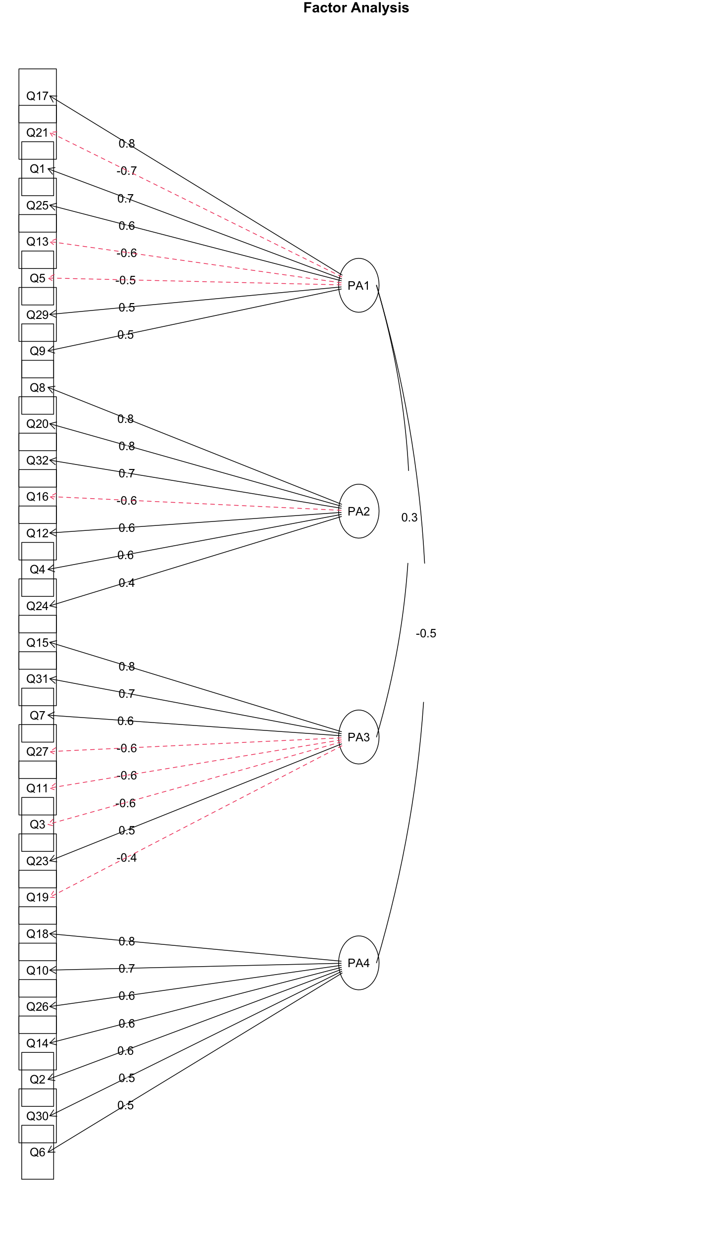
1 2 3 4 5 6 7 8 9 10 11 efa_4_pa <- fa( analysis_data, nfactors= 4 , rotate= "promax" , fm= "pa" ) efa_4_pa$ Vaccounted efa_4_pa$ communality efa_4_pa$ loadings print( efa_4_pa$ loadings, cutoff= 0.3 )
1 2 3 4 5 6 7 8 9 10 11 12 13 14 15 16 17 18 19 20 21 22 23 24 25 26 27 28 29 30 31 32 33 34 35 36 37 38 39 40 41 42 43 44 45 46 47 48 49 50 51 > efa_4_pa$ Vaccounted PA1 PA2 PA4 PA3 SS loadings 3.6326482 3.15732774 3.0501600 3.04880469 Proportion Var 0.1135203 0.09866649 0.0953175 0.09527515 Cumulative Var 0.1135203 0.21218675 0.3075042 0.40277940 Proportion Explained 0.2818423 0.24496410 0.2366494 0.23654424 Cumulative Proportion 0.2818423 0.52680636 0.7634558 1.00000000 > efa_4_pa$ communality Q1 Q2 Q3 Q4 Q5 Q6 Q7 Q8 Q9 Q10 Q11 Q12 Q13 0.4900625 0.3937478 0.4067060 0.3584038 0.3256476 0.2662986 0.3822206 0.6101605 0.2693080 0.5384912 0.3172389 0.3925288 0.4219459 Q14 Q15 Q16 Q17 Q18 Q19 Q20 Q21 Q22 Q23 Q24 Q25 Q26 0.4532441 0.5764920 0.3976837 0.6248901 0.6294796 0.3836804 0.5833695 0.5209850 0.1843002 0.2696753 0.1921420 0.3905649 0.4716011 Q27 Q28 Q29 Q30 Q31 Q32 0.3483654 0.2010546 0.3486561 0.1874059 0.4625831 0.4900075 > print( efa_4_pa$ loadings, cutoff= 0.3 ) Loadings: PA1 PA2 PA4 PA3 Q1 0.700 Q2 0.592 Q3 - 0.566 Q4 0.601 Q5 - 0.546 Q6 0.457 Q7 0.655 Q8 0.789 Q9 0.509 Q10 0.765 Q11 - 0.594 Q12 0.627 Q13 - 0.626 Q14 0.606 Q15 0.782 Q16 - 0.620 Q17 0.815 Q18 0.858 Q19 - 0.427 Q20 0.762 Q21 - 0.731 Q22 Q23 0.478 Q24 0.432 Q25 0.639 Q26 0.653 Q27 - 0.611 Q28 Q29 0.548 Q30 0.482 Q31 0.674 Q32 0.681
可以看出,总体方差解释率为40.277940%
有两个变量Q22与Q28在所有因素上的载荷绝对值都小于0.3。并且Q22的共同度为0.1843002,Q28的共同度为0.2010546。
为了避免误删的情况,一次删除一个变量 ,先删除共同度更低的Q22
1 2 3 4 5 6 7 8 9 10 11 12 13 14 15 16 17 analysis_data1 <- subset( analysis_data, select = - Q22) names ( analysis_data1) efa_4_pa1 <- fa( analysis_data1, nfactors= 4 , rotate= "promax" , fm= "pa" ) efa_4_pa1$ Vaccounted efa_4_pa1$ communality efa_4_pa1$ loadings print( efa_4_pa1$ loadings, cutoff= 0.3 ) plot( efa_4_pa1) fa.diagram( efa_4_pa1)
1 2 3 4 5 6 7 8 9 10 11 12 13 14 15 16 17 18 19 20 21 22 23 24 25 26 27 28 29 30 31 32 33 34 35 36 37 38 39 40 41 42 43 44 45 46 47 48 49 > efa_4_pa1$ Vaccounted PA1 PA2 PA3 PA4 SS loadings 3.5893385 3.1448807 3.04123134 2.92815052 Proportion Var 0.1157851 0.1014478 0.09810424 0.09445647 Cumulative Var 0.1157851 0.2172329 0.31533711 0.40979358 Proportion Explained 0.2825450 0.2475582 0.23939915 0.23049768 Cumulative Proportion 0.2825450 0.5301032 0.76950232 1.00000000 > efa_4_pa1$ communality Q1 Q2 Q3 Q4 Q5 Q6 Q7 Q8 Q9 Q10 Q11 Q12 Q13 0.4863391 0.3795585 0.4091628 0.3578021 0.3240189 0.2766300 0.3825274 0.6092897 0.2706913 0.5401742 0.3174019 0.3949205 0.4275838 Q14 Q15 Q16 Q17 Q18 Q19 Q20 Q21 Q23 Q24 Q25 Q26 Q27 0.4403981 0.5756366 0.3959852 0.6258198 0.6288677 0.3899786 0.5801802 0.5219272 0.2694124 0.1931119 0.3943182 0.4680189 0.3528202 Q28 Q29 Q30 Q31 Q32 0.2060787 0.3450362 0.1908110 0.4578422 0.4912575 > print( efa_4_pa1$ loadings, cutoff= 0.3 ) Loadings: PA1 PA2 PA3 PA4 Q1 0.693 Q2 0.570 Q3 - 0.566 Q4 0.598 Q5 - 0.541 Q6 0.461 Q7 0.651 Q8 0.785 Q9 0.505 Q10 0.752 Q11 - 0.591 Q12 0.625 Q13 - 0.622 Q14 0.586 Q15 0.776 Q16 - 0.616 Q17 0.806 Q18 0.841 Q19 - 0.430 Q20 0.758 Q21 - 0.724 Q23 0.476 Q24 0.429 Q25 0.634 Q26 0.639 Q27 - 0.610 Q28 Q29 0.539 Q30 0.476 Q31 0.667 Q32 0.680
可以看出,总体方差解释率为40.979358%
变量Q28在所有因素上的载荷绝对值小于0.3,Q28的共同度为0.2060787。
继续删除Q28变量
1 2 3 4 5 6 7 8 9 10 11 12 13 14 15 16 17 18 analysis_data2 <- subset( analysis_data1, select = - Q28) names ( analysis_data2) efa_4_pa2 <- fa( analysis_data2, nfactors= 4 , rotate= "promax" , fm= "pa" ) efa_4_pa2$ Vaccounted efa_4_pa2$ communality efa_4_pa2$ loadings print( efa_4_pa2$ loadings, cutoff= 0.3 ) plot( efa_4_pa2) fa.diagram( efa_4_pa2)
1 2 3 4 5 6 7 8 9 10 11 12 13 14 15 16 17 18 19 20 21 22 23 24 25 26 27 28 29 30 31 32 33 34 35 36 37 38 39 40 41 42 43 44 45 46 47 48 49 > efa_4_pa2$ Vaccounted PA1 PA2 PA3 PA4 SS loadings 3.5828806 3.0766135 2.99839031 2.84177976 Proportion Var 0.1194294 0.1025538 0.09994634 0.09472599 Cumulative Var 0.1194294 0.2219831 0.32192948 0.41665547 Proportion Explained 0.2866381 0.2461357 0.23987767 0.22734849 Cumulative Proportion 0.2866381 0.5327738 0.77265151 1.00000000 > efa_4_pa2$ communality Q1 Q2 Q3 Q4 Q5 Q6 Q7 Q8 Q9 Q10 Q11 Q12 Q13 0.4862573 0.3824251 0.4032269 0.3536933 0.3241615 0.2812596 0.3745370 0.6094749 0.2703332 0.5315761 0.3167107 0.3900420 0.4270932 Q14 Q15 Q16 Q17 Q18 Q19 Q20 Q21 Q23 Q24 Q25 Q26 Q27 0.4543375 0.5865768 0.4022270 0.6254822 0.6306127 0.3890294 0.5902971 0.5227965 0.2737261 0.1899345 0.3935340 0.4567565 0.3432978 Q29 Q30 Q31 Q32 0.3456581 0.1904744 0.4630060 0.4911267 > print( efa_4_pa2$ loadings, cutoff= 0.3 ) Loadings: PA1 PA2 PA3 PA4 Q1 0.693 Q2 0.566 Q3 - 0.560 Q4 0.589 Q5 - 0.540 Q6 0.459 Q7 0.640 Q8 0.776 Q9 0.504 Q10 0.737 Q11 - 0.585 Q12 0.612 Q13 - 0.621 Q14 0.591 Q15 0.776 Q16 - 0.613 Q17 0.807 Q18 0.831 Q19 - 0.432 Q20 0.757 Q21 - 0.722 Q23 0.477 Q24 0.423 Q25 0.629 Q26 0.620 Q27 - 0.598 Q29 0.539 Q30 0.467 Q31 0.662 Q32 0.673
1 2 3 4 5 6 > efa_4_pa2$ score.cor [ , 1 ] [ , 2 ] [ , 3 ] [ , 4 ] [ 1 , ] 1.0000000 - 0.1472319 0.2644861 - 0.4064475 [ 2 , ] - 0.1472319 1.0000000 - 0.1725307 0.1851080 [ 3 , ] 0.2644861 - 0.1725307 1.0000000 - 0.1787275 [ 4 , ] - 0.4064475 0.1851080 - 0.1787275 1.0000000
可以根据每个因素下的题目的意义给因素命名
CFA
导入包与数据
1 2 3 4 5 6 7 8 9 10 11 library( lavaan) library( semPlot) setwd( "/Users/nanxu/研究生课程作业/心理统计/课件数据/8第八章 验证性因素分析/" ) data <- read.table( "./8_1.dat" , header = FALSE , sep = "" , na.strings = "NA" ) names ( data) dim ( data)
数据介绍
后三列数据分别是被试编码、被试年龄以及性别
探索性因素分析
第一次CFA
模型识别:待估计的参数数量t=11(因素载荷)+11(误差项方差)+1(两个因素的相关)=23 < (模型协方差矩阵的元素数)q ( q + 1 ) 2 \frac{q(q+1)}{2} 2 q ( q + 1 )
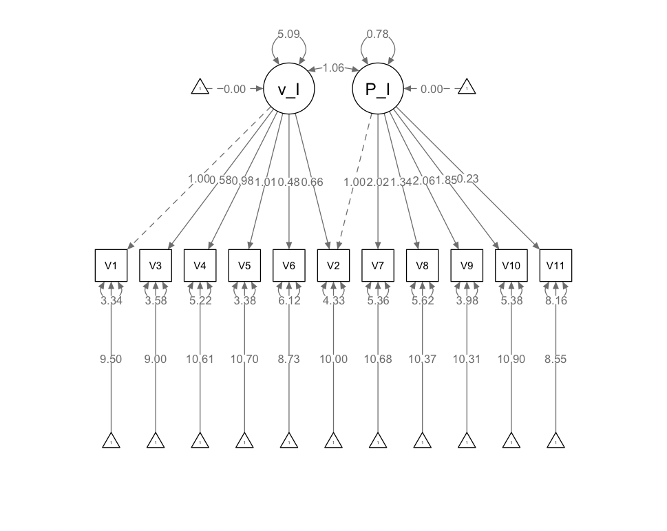
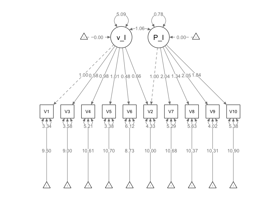
1 2 3 4 5 6 7 8 9 10 11 12 13 14 15 16 17 18 19 20 21 22 23 24 25 26 27 28 29 30 31 32 model1 <- ' # 定义潜变量 verbal_IQ verbal_IQ =~ V1 + V2 + V3 + V4 + V5 + V6 # 定义潜变量 Performance_IQ Performance_IQ =~ V7 + V8 + V9 + V10 + V11 # 显式请求截距 V1 ~1 V2 ~1 V3 ~1 V4 ~1 V5 ~1 V6 ~1 V7 ~1 V8 ~1 V9 ~1 V10 ~1 V11 ~1 ' fit1 <- cfa( model1, data= data) summary( fit1, fit.measures = TRUE , standardized= TRUE , rsquare = TRUE ) modificationIndices( fit1, sort = TRUE , minimum.value = 4.0 ) semPaths( fit1, whatLabels= "est" , layout= "tree" , edge.label.cex= 0.8 , node.label.cex= 0.9 )
模型拟合结果
卡方值
1 2 3 4 5 6 7 8 9 10 11 Model Test User Model: Test statistic 70.640 Degrees of freedom 43 P- value ( Chi- square) 0.005 Model Test Baseline Model: Test statistic 519.204 Degrees of freedom 55 P- value 0.000
似然值与信息标准指数
1 2 3 4 5 6 7 8 Loglikelihood and Information Criteria: Loglikelihood user model ( H0) - 4491.822 Loglikelihood unrestricted model ( H1) - 4456.502 Akaike ( AIC) 9051.643 Bayesian ( BIC) 9159.246 Sample- size adjusted Bayesian ( SABIC) 9051.579
相对拟合指数(比较拟合指数CFI、非标准拟合指数TLI)与绝对拟合指数(近似误差均方根RMSEA)
1 2 3 4 5 6 7 8 9 10 11 12 13 14 15 16 17 User Model versus Baseline Model: Comparative Fit Index ( CFI) 0.940 Tucker- Lewis Index ( TLI) 0.924 Root Mean Square Error of Approximation: RMSEA 0.061 90 Percent confidence interval - lower 0.033 90 Percent confidence interval - upper 0.085 P- value H_0: RMSEA <= 0.050 0.233 P- value H_0: RMSEA >= 0.080 0.103 Standardized Root Mean Square Residual: SRMR 0.054
模型的RMSEA为0.061小于0.08,CFI为0.940,TLI为0.924,均大于0.9,表明模型拟合结果良好。
模型原始估计结果
因素载荷结果的估计值、标准误差、z分数以及统计显著性检验结果,方差标准化的结果Std.all
默认采用固定因素载荷为1的方法设定潜变量的量尺,采用每个潜变量的第一个观测变量的因素载荷为1
1 2 3 4 5 6 7 8 9 10 11 12 13 14 15 Latent Variables: Estimate Std.Err z- value P( > | z| ) Std.lv Std.all verbal_IQ = ~ V1 1.000 2.206 0.760 V2 0.926 0.108 8.609 0.000 2.042 0.691 V3 0.589 0.084 7.013 0.000 1.300 0.565 V4 1.012 0.115 8.764 0.000 2.232 0.703 V5 1.020 0.107 9.548 0.000 2.250 0.770 V6 0.477 0.099 4.805 0.000 1.053 0.390 Performance_IQ = ~ V7 1.000 1.742 0.595 V8 0.719 0.156 4.614 0.000 1.253 0.473 V9 1.060 0.187 5.675 0.000 1.846 0.683 V10 0.921 0.177 5.215 0.000 1.605 0.566 V11 0.119 0.147 0.810 0.418 0.207 0.072
可以看出,X11在潜变量F2上的标准化因素载荷仅为0.072,且没有达到显著水平
潜变量的相关的估计值、标准误差、z分数以及统计显著性检验结果,方差标准化的结果Std.all
1 2 3 4 Covariances: Estimate Std.Err z- value P( > | z| ) Std.lv Std.all verbal_IQ ~ ~ Performance_IQ 2.263 0.515 4.397 0.000 0.589 0.589
截距的估计值、标准误差、z分数以及统计显著性检验结果,方差标准化的结果Std.all
1 2 3 4 5 6 7 8 9 10 11 12 13 Intercepts: Estimate Std.Err z- value P( > | z| ) Std.lv Std.all .V1 9.497 0.220 43.264 0.000 9.497 3.270 .V2 10.000 0.224 44.740 0.000 10.000 3.382 .V3 9.000 0.174 51.758 0.000 9.000 3.913 .V4 10.611 0.240 44.220 0.000 10.611 3.343 .V5 10.703 0.221 48.416 0.000 10.703 3.660 .V6 8.731 0.204 42.837 0.000 8.731 3.238 .V7 10.680 0.221 48.288 0.000 10.680 3.650 .V8 10.371 0.200 51.734 0.000 10.371 3.911 .V9 10.314 0.204 50.496 0.000 10.314 3.817 .V10 10.903 0.214 50.860 0.000 10.903 3.845 .V11 8.549 0.216 39.487 0.000 8.549 2.985
误差的方差与潜变量的方差的估计值、标准误差、z分数以及统计显著性检验结果,方差标准化的结果Std.all
1 2 3 4 5 6 7 8 9 10 11 12 13 14 15 Variances: Estimate Std.Err z- value P( > | z| ) Std.lv Std.all .V1 3.566 0.507 7.034 0.000 3.566 0.423 .V2 4.572 0.585 7.815 0.000 4.572 0.523 .V3 3.602 0.420 8.571 0.000 3.602 0.681 .V4 5.096 0.662 7.702 0.000 5.096 0.506 .V5 3.487 0.506 6.886 0.000 3.487 0.408 .V6 6.162 0.680 9.056 0.000 6.162 0.848 .V7 5.526 0.757 7.296 0.000 5.526 0.646 .V8 5.463 0.658 8.298 0.000 5.463 0.777 .V9 3.894 0.640 6.083 0.000 3.894 0.533 .V10 5.467 0.719 7.600 0.000 5.467 0.680 .V11 8.159 0.874 9.335 0.000 8.159 0.995 verbal_IQ 4.867 0.883 5.514 0.000 1.000 1.000 Performance_IQ 3.035 0.844 3.593 0.000 1.000 1.000
R2 结果
R2 结果为每道题标准化因素载荷的平凡,描述了题目信度的高低
1 2 3 4 5 6 7 8 9 10 11 12 13 R- Square: Estimate V1 0.577 V2 0.477 V3 0.319 V4 0.494 V5 0.592 V6 0.152 V7 0.354 V8 0.223 V9 0.467 V10 0.320 V11 0.005
修正指数结果
1 2 modificationIndices( fit1, sort = TRUE , minimum.value = 4.0 )
修正指数结果部分呈现了所有可能路径的修正指数值mi、自由估计该参数时可能的估计值epc、使用连续潜变量的方差标准化的估计值sepc.lv、使用连续潜变量及背景变量和结果变量的方差进行标准化的估计值sepc.all
1 2 3 4 5 6 7 8 9 10 11 lhs op rhs mi epc sepc.lv sepc.all sepc.nox 45 Performance_IQ = ~ V2 9.823 0.538 0.937 0.317 0.317 75 V3 ~ ~ V10 6.362 - 0.945 - 0.945 - 0.213 - 0.213 50 V1 ~ ~ V2 5.221 - 0.985 - 0.985 - 0.244 - 0.244 94 V6 ~ ~ V11 4.927 1.207 1.207 0.170 0.170 64 V2 ~ ~ V7 4.685 0.969 0.969 0.193 0.193 98 V7 ~ ~ V11 4.575 - 1.225 - 1.225 - 0.182 - 0.182 44 Performance_IQ = ~ V1 4.477 - 0.342 - 0.596 - 0.205 - 0.205 53 V1 ~ ~ V5 4.403 0.912 0.912 0.259 0.259 86 V5 ~ ~ V8 4.146 - 0.798 - 0.798 - 0.183 - 0.183 51 V1 ~ ~ V3 4.133 0.697 0.697 0.194 0.194
看出V2可能测量了Performance_IQ这个因素
修正后的第二次CFA
1 2 3 4 5 6 7 8 9 10 11 12 13 14 15 16 17 18 19 20 21 22 23 24 25 26 27 model2 <- ' # 定义潜变量 verbal_IQ verbal_IQ =~ V1 + V2 + V3 + V4 + V5 + V6 # 定义潜变量 Performance_IQ Performance_IQ =~ V2 + V7 + V8 + V9 + V10 + V11 # 显式请求截距 V1 ~1 V2 ~1 V3 ~1 V4 ~1 V5 ~1 V6 ~1 V7 ~1 V8 ~1 V9 ~1 V10 ~1 V11 ~1 ' fit2 <- cfa( model2, data= data) summary( fit2, fit.measures = TRUE , standardized= TRUE , rsquare = TRUE ) semPaths( fit2, whatLabels= "est" , layout= "tree" , edge.label.cex= 0.8 , node.label.cex= 0.9 )
1 2 3 4 5 6 7 8 9 10 11 12 13 14 15 16 17 18 19 20 21 22 23 24 25 26 27 28 29 30 31 32 33 34 35 36 37 Model Test User Model: Test statistic 60.642 Degrees of freedom 42 P- value ( Chi- square) 0.031 Model Test Baseline Model: Test statistic 519.204 Degrees of freedom 55 P- value 0.000 User Model versus Baseline Model: Comparative Fit Index ( CFI) 0.960 Tucker- Lewis Index ( TLI) 0.947 Loglikelihood and Information Criteria: Loglikelihood user model ( H0) - 4486.823 Loglikelihood unrestricted model ( H1) - 4456.502 Akaike ( AIC) 9043.645 Bayesian ( BIC) 9154.413 Sample- size adjusted Bayesian ( SABIC) 9043.579 Root Mean Square Error of Approximation: RMSEA 0.050 90 Percent confidence interval - lower 0.016 90 Percent confidence interval - upper 0.077 P- value H_0: RMSEA <= 0.050 0.465 P- value H_0: RMSEA >= 0.080 0.031 Standardized Root Mean Square Residual: SRMR 0.050
1 2 3 4 5 6 7 8 9 10 11 12 13 14 15 16 17 18 19 20 21 22 23 24 25 26 27 28 29 30 31 32 33 34 35 36 37 38 39 40 41 42 43 44 45 46 47 48 49 50 51 52 53 54 55 56 57 58 59 60 61 62 63 64 65 66 Latent Variables: Estimate Std.Err z- value P( > | z| ) Std.lv Std.all verbal_IQ = ~ V1 1.000 2.256 0.777 V2 0.661 0.118 5.606 0.000 1.491 0.504 V3 0.579 0.082 7.101 0.000 1.307 0.568 V4 0.977 0.112 8.751 0.000 2.205 0.695 V5 1.008 0.103 9.739 0.000 2.273 0.777 V6 0.476 0.097 4.918 0.000 1.075 0.399 Performance_IQ = ~ V2 1.000 0.884 0.299 V7 2.024 0.657 3.080 0.002 1.790 0.612 V8 1.345 0.470 2.862 0.004 1.189 0.448 V9 2.062 0.662 3.112 0.002 1.823 0.675 V10 1.847 0.606 3.048 0.002 1.633 0.576 V11 0.227 0.294 0.772 0.440 0.200 0.070 Covariances: Estimate Std.Err z- value P( > | z| ) Std.lv Std.all verbal_IQ ~ ~ Performance_IQ 1.064 0.380 2.795 0.005 0.533 0.533 Intercepts: Estimate Std.Err z- value P( > | z| ) Std.lv Std.all .V1 9.497 0.220 43.264 0.000 9.497 3.270 .V2 10.000 0.224 44.740 0.000 10.000 3.382 .V3 9.000 0.174 51.758 0.000 9.000 3.913 .V4 10.611 0.240 44.220 0.000 10.611 3.343 .V5 10.703 0.221 48.416 0.000 10.703 3.660 .V6 8.731 0.204 42.837 0.000 8.731 3.238 .V7 10.680 0.221 48.288 0.000 10.680 3.650 .V8 10.371 0.200 51.734 0.000 10.371 3.911 .V9 10.314 0.204 50.496 0.000 10.314 3.817 .V10 10.903 0.214 50.860 0.000 10.903 3.845 .V11 8.549 0.216 39.487 0.000 8.549 2.985 Variances: Estimate Std.Err z- value P( > | z| ) Std.lv Std.all .V1 3.343 0.502 6.665 0.000 3.343 0.396 .V2 4.331 0.554 7.819 0.000 4.331 0.495 .V3 3.584 0.420 8.533 0.000 3.584 0.677 .V4 5.217 0.675 7.726 0.000 5.217 0.518 .V5 3.383 0.508 6.655 0.000 3.383 0.396 .V6 6.116 0.677 9.032 0.000 6.116 0.841 .V7 5.358 0.741 7.231 0.000 5.358 0.626 .V8 5.620 0.663 8.480 0.000 5.620 0.799 .V9 3.979 0.623 6.385 0.000 3.979 0.545 .V10 5.376 0.707 7.603 0.000 5.376 0.668 .V11 8.162 0.874 9.337 0.000 8.162 0.995 verbal_IQ 5.090 0.899 5.659 0.000 1.000 1.000 Performance_IQ 0.782 0.470 1.662 0.097 1.000 1.000 R- Square: Estimate V1 0.604 V2 0.505 V3 0.323 V4 0.482 V5 0.604 V6 0.159 V7 0.374 V8 0.201 V9 0.455 V10 0.332 V11 0.005
可以看出X11的因素载荷是不显著的,且标准化的载荷值只有0.070。可以考虑删除X11
比较模型拟合指数
模型2是在模型1的基础上增加了参数,两个模型呈嵌套关系,可以进行拟合程度比较。
1 2 3 4 5 Chi- Squared Difference Test Df AIC BIC Chisq Chisq diff RMSEA Df diff Pr( > Chisq) fit2 42 9043.6 9154.4 60.642 fit1 43 9051.6 9159.2 70.640 9.998 0.22675 1 0.001567 * *
可以看出两个模型的卡方值的差值Chisq diff为9.998,自由度的差值为1,表明两个模型的差异显著。模型二的拟合指数AIC、BIC、RMSEA、CFI、TLI优于模型1。
修正后的第三次CFA
1 2 3 4 5 6 7 8 9 10 11 12 13 14 15 16 17 18 19 20 21 22 23 24 25 26 model3 <- ' # 定义潜变量 verbal_IQ verbal_IQ =~ V1 + V2 + V3 + V4 + V5 + V6 # 定义潜变量 Performance_IQ Performance_IQ =~ V2 + V7 + V8 + V9 + V10 # 显式请求截距 V1 ~1 V2 ~1 V3 ~1 V4 ~1 V5 ~1 V6 ~1 V7 ~1 V8 ~1 V9 ~1 V10 ~1 ' fit3 <- cfa( model3, data= data) summary( fit3, fit.measures = TRUE , standardized= TRUE , rsquare = TRUE ) semPaths( fit3, whatLabels= "est" , layout= "tree" , edge.label.cex= 0.8 , node.label.cex= 0.9 )
1 2 3 4 5 6 7 8 9 10 11 12 13 14 15 16 17 18 19 20 21 22 23 24 25 26 27 28 29 30 31 32 33 34 35 36 37 Model Test User Model: Test statistic 45.276 Degrees of freedom 33 P- value ( Chi- square) 0.075 Model Test Baseline Model: Test statistic 503.222 Degrees of freedom 45 P- value 0.000 User Model versus Baseline Model: Comparative Fit Index ( CFI) 0.973 Tucker- Lewis Index ( TLI) 0.963 Loglikelihood and Information Criteria: Loglikelihood user model ( H0) - 4054.684 Loglikelihood unrestricted model ( H1) - 4032.046 Akaike ( AIC) 8173.368 Bayesian ( BIC) 8274.642 Sample- size adjusted Bayesian ( SABIC) 8173.308 Root Mean Square Error of Approximation: RMSEA 0.046 90 Percent confidence interval - lower 0.000 90 Percent confidence interval - upper 0.077 P- value H_0: RMSEA <= 0.050 0.549 P- value H_0: RMSEA >= 0.080 0.033 Standardized Root Mean Square Residual: SRMR 0.045
1 2 3 4 5 6 7 8 9 10 11 12 13 14 15 16 17 18 19 20 21 22 23 24 25 26 27 28 29 30 31 32 33 34 35 36 37 38 39 40 41 42 43 44 45 46 47 48 49 50 51 52 53 54 55 56 57 58 59 60 61 Latent Variables: Estimate Std.Err z- value P( > | z| ) Std.lv Std.all verbal_IQ = ~ V1 1.000 2.256 0.777 V2 0.661 0.118 5.608 0.000 1.491 0.504 V3 0.579 0.082 7.099 0.000 1.306 0.568 V4 0.977 0.112 8.755 0.000 2.206 0.695 V5 1.007 0.103 9.738 0.000 2.273 0.777 V6 0.476 0.097 4.916 0.000 1.074 0.398 Performance_IQ = ~ V2 1.000 0.885 0.299 V7 2.041 0.661 3.088 0.002 1.807 0.618 V8 1.340 0.468 2.863 0.004 1.186 0.447 V9 2.045 0.657 3.114 0.002 1.811 0.670 V10 1.843 0.604 3.051 0.002 1.632 0.575 Covariances: Estimate Std.Err z- value P( > | z| ) Std.lv Std.all verbal_IQ ~ ~ Performance_IQ 1.064 0.381 2.797 0.005 0.533 0.533 Intercepts: Estimate Std.Err z- value P( > | z| ) Std.lv Std.all .V1 9.497 0.220 43.264 0.000 9.497 3.270 .V2 10.000 0.224 44.740 0.000 10.000 3.382 .V3 9.000 0.174 51.758 0.000 9.000 3.913 .V4 10.611 0.240 44.220 0.000 10.611 3.343 .V5 10.703 0.221 48.416 0.000 10.703 3.660 .V6 8.731 0.204 42.837 0.000 8.731 3.238 .V7 10.680 0.221 48.288 0.000 10.680 3.650 .V8 10.371 0.200 51.734 0.000 10.371 3.911 .V9 10.314 0.204 50.496 0.000 10.314 3.817 .V10 10.903 0.214 50.860 0.000 10.903 3.845 Variances: Estimate Std.Err z- value P( > | z| ) Std.lv Std.all .V1 3.342 0.502 6.662 0.000 3.342 0.396 .V2 4.329 0.554 7.815 0.000 4.329 0.495 .V3 3.585 0.420 8.534 0.000 3.585 0.677 .V4 5.213 0.675 7.724 0.000 5.213 0.517 .V5 3.385 0.508 6.658 0.000 3.385 0.396 .V6 6.117 0.677 9.032 0.000 6.117 0.841 .V7 5.295 0.740 7.156 0.000 5.295 0.619 .V8 5.626 0.663 8.482 0.000 5.626 0.800 .V9 4.022 0.624 6.445 0.000 4.022 0.551 .V10 5.379 0.708 7.602 0.000 5.379 0.669 verbal_IQ 5.091 0.899 5.660 0.000 1.000 1.000 Performance_IQ 0.784 0.471 1.665 0.096 1.000 1.000 R- Square: Estimate V1 0.604 V2 0.505 V3 0.323 V4 0.483 V5 0.604 V6 0.159 V7 0.381 V8 0.200 V9 0.449 V10 0.331
比较模型拟合指数
1 2 3 4 5 6 Chi- Squared Difference Test Df AIC BIC Chisq Chisq diff RMSEA Df diff Pr( > Chisq) fit3 33 8173.4 8274.6 45.276 fit2 42 9043.6 9154.4 60.642 15.365 0.063572 9 0.081379 . fit1 43 9051.6 9159.2 70.640 9.998 0.226753 1 0.001567 * *
模型三与模型二保焊的变量不同,不具有嵌套关系。只需要参考拟合指数AIC、BIC、RMSEA、CFI、TLI,表明模型三优于模型二。
等价性检验
对不同性别的测验等价性进行检验
1 2 3 4 analysis_data_withgender$ V14 <- factor( analysis_data_withgender$ V14, levels = c ( 0 , 1 ) , labels = c ( "male" , "female" ) ) table( analysis_data_withgender$ V14)
使用最终确定的模型三作为等价性检验模型
1 2 3 4 5 6 7 8 9 10 11 12 13 14 15 16 17 18 19 20 model3 <- ' # 定义潜变量 verbal_ IQ verbal_IQ =~ V1 + V2 + V3 + V4 + V5 + V6 # 定义潜变量 Performance_IQ Performance_IQ =~ V2 + V7 + V8 + V9 + V10 # 显式请求截距 V1 ~1 V2 ~1 V3 ~1 V4 ~1 V5 ~1 V6 ~1 V7 ~1 V8 ~1 V9 ~1 V10 ~1 '
不同性别分别拟合模型
1 2 3 4 5 6 7 8 9 10 11 data_male <- subset( data, V14 == "male" ) data_female <- subset( data, V14 == "female" ) fit_male <- cfa( model3, data = data_male) summary( fit_male, fit.measures = TRUE , standardized = TRUE , rsquare = TRUE ) fit_female <- cfa( model3, data = data_female) summary( fit_female, fit.measures = TRUE , standardized = TRUE , rsquare = TRUE )
1 2 3 4 5 6 7 8 9 10 11 12 13 14 15 16 17 18 19 20 21 22 23 24 25 26 27 28 29 30 > summary( fit_male, fit.measures = TRUE , standardized = TRUE , rsquare = TRUE ) User Model versus Baseline Model: Comparative Fit Index ( CFI) 0.910 Tucker- Lewis Index ( TLI) 0.877 Root Mean Square Error of Approximation: RMSEA 0.081 90 Percent confidence interval - lower 0.033 90 Percent confidence interval - upper 0.122 P- value H_0: RMSEA <= 0.050 0.121 P- value H_0: RMSEA >= 0.080 0.546 > summary( fit_female, fit.measures = TRUE , standardized = TRUE , rsquare = TRUE ) User Model versus Baseline Model: Comparative Fit Index ( CFI) 1.000 Tucker- Lewis Index ( TLI) 1.030 Root Mean Square Error of Approximation: RMSEA 0.000 90 Percent confidence interval - lower 0.000 90 Percent confidence interval - upper 0.058 P- value H_0: RMSEA <= 0.050 0.920 P- value H_0: RMSEA >= 0.080 0.008
可以看出男生组RMSEA为0.081,CFI值为0.910,TLI值为0.877;女生组RMSEA为0.000,CFI值为1.000,TLI值为1.030,表明两组模型都拟合良好
因素模式相同模型(基线模型)
1 2 3 configural_model <- cfa( model3, data= data, group= "V14" ) summary( configural_model, fit.measures= TRUE , standardized= TRUE , rsquare = TRUE )
1 2 3 4 5 6 7 8 9 10 11 12 13 14 15 16 17 18 19 20 21 22 23 24 25 26 27 28 29 30 31 32 33 34 35 36 37 38 39 40 41 Model Test User Model: Test statistic 79.129 Degrees of freedom 66 P- value ( Chi- square) 0.129 Test statistic for each group: female 27.457 male 51.672 Model Test Baseline Model: Test statistic 548.746 Degrees of freedom 90 P- value 0.000 User Model versus Baseline Model: Comparative Fit Index ( CFI) 0.971 Tucker- Lewis Index ( TLI) 0.961 Loglikelihood and Information Criteria: Loglikelihood user model ( H0) - 4044.360 Loglikelihood unrestricted model ( H1) - 4004.796 Akaike ( AIC) 8216.720 Bayesian ( BIC) 8419.266 Sample- size adjusted Bayesian ( SABIC) 8216.598 Root Mean Square Error of Approximation: RMSEA 0.048 90 Percent confidence interval - lower 0.000 90 Percent confidence interval - upper 0.083 P- value H_0: RMSEA <= 0.050 0.516 P- value H_0: RMSEA >= 0.080 0.068 Standardized Root Mean Square Residual: SRMR 0.057
可以看出RMSEA值为0.048,CFI的值为0.971,TLI的值为0.961,表明模型拟合较好。该模型作为基线模型,用于检验其他等价性条件是否满足。
因素载荷等价模型(弱等价性)
不同组的观测变量与对应的潜变量之间的因素载荷的值是相等的
1 2 3 metric_model <- cfa( model3, data= analysis_data_withgender, group= "V14" , group.equal= "loadings" ) summary( metric_model, fit.measures= TRUE , standardized= TRUE , rsquare = TRUE )
1 2 3 4 5 6 7 > anova( configural_model, metric_model) Chi- Squared Difference Test Df AIC BIC Chisq Chisq diff RMSEA Df diff Pr( > Chisq) configural_model 66 8216.7 8419.3 79.129 metric_model 75 8205.9 8380.0 86.297 7.1688 0 9 0.6196
弱等价性模型嵌套于基线模型,可以使用嵌套模型的比较方法。
可以看出两个模型的卡方值的差值Chisq diff为7.1688,自由度的差值Df diff为9,表明两个模型的卡方差异不显著。可以接受弱等价模型,即认为不同性别之间满足因素载荷等价条件。
截距等价性模型(强等价性)
不同组的观测变量的截距相等
1 2 3 scalar_model <- cfa( model3, data= analysis_data_withgender, group= "V14" , group.equal= c ( "loadings" , "intercepts" ) ) summary( scalar_model, fit.measures= TRUE , standardized= TRUE , rsquare = TRUE )
1 2 3 4 5 6 7 8 > anova( configural_model, metric_model, scalar_model) Chi- Squared Difference Test Df AIC BIC Chisq Chisq diff RMSEA Df diff Pr( > Chisq) configural_model 66 8216.7 8419.3 79.129 metric_model 75 8205.9 8380.0 86.297 7.1688 0 9 0.6196 scalar_model 83 8193.3 8342.0 89.687 3.3898 0 8 0.9076
强等价性模型嵌套于弱等价性模型,可以使用嵌套模型的比较方法。
可以看出两个模型的卡方值的差值Chisq diff为3.3898,自由度的差值Df diff为8,表明两个模型的卡方差异不显著。可以接受强等价模型,即认为不同性别之间满足截距等价条件。
误差方差等价模型
假定来自不同组的误差方差相等
1 2 3 error_variance_model <- cfa( model3, data= analysis_data_withgender, group= "V14" , group.equal= c ( "loadings" , "intercepts" , "residuals" ) ) summary( error_variance_model, fit.measures= TRUE , standardized= TRUE , rsquare = TRUE )
1 2 3 4 5 6 7 8 9 > anova( configural_model, metric_model, scalar_model, error_variance_model) Chi- Squared Difference Test Df AIC BIC Chisq Chisq diff RMSEA Df diff Pr( > Chisq) configural_model 66 8216.7 8419.3 79.129 metric_model 75 8205.9 8380.0 86.297 7.1688 0 9 0.6196 scalar_model 83 8193.3 8342.0 89.687 3.3898 0 8 0.9076 error_variance_model 93 8178.4 8295.5 94.812 5.1252 0 10 0.8827
误差方差等价模型嵌套于强等价性模型,可以使用嵌套模型的比较方法。
可以看出两个模型的卡方值的差值Chisq diff为5.1252,自由度的差值Df diff为10,表明两个模型的卡方差异不显著。可以接受误差方差等价模型,即认为不同性别之间满足误差方差等价条件。
潜变量方差等价模型
假定来自不同组的误差方差相等,不同组的误差协方差相等
1 2 3 latent_variance_model <- cfa( model3, data= analysis_data_withgender, group= "V14" , group.equal= c ( "loadings" , "intercepts" , "residuals" , "lv.variances" ) ) summary( latent_variance_model, fit.measures= TRUE , standardized= TRUE , rsquare = TRUE )
1
2
3
4
5
6
7
8
9
10
> anova( configural_model, metric_model, scalar_model, error_variance_model, latent_variance_model) Chi- Squared Difference Test Df AIC BIC Chisq Chisq diff RMSEA Df diff Pr( > Chisq) configural_model 66 8216.7 8419.3 79.129 metric_model 75 8205.9 8380.0 86.297 7.1688 0.000000 9 0.6196 scalar_model 83 8193.3 8342.0 89.687 3.3898 0.000000 8 0.9076 error_variance_model 93 8178.4 8295.5 94.812 5.1252 0.000000 10 0.8827 latent_variance_model 95 8177.7 8288.5 98.131 3.3185 0.086801 2 0.1903
潜变量方差等价模型嵌套于误差方差等价模型,可以使用嵌套模型的比较方法。
可以看出两个模型的卡方值的差值Chisq diff为3.3185,自由度的差值Df diff为2,表明两个模型的卡方差异不显著。可以接受潜变量方差等价模型,即认为不同性别之间满足潜变量方差等价条件。
潜变量协方差矩阵等价模型
1 2 3 latent_covariance_model <- cfa( model3, data= analysis_data_withgender, group= "V14" , group.equal= c ( "loadings" , "intercepts" , "residuals" , "lv.variances" , "lv.covariances" ) ) summary( latent_covariance_model, fit.measures= TRUE , standardized= TRUE , rsquare = TRUE )
1 2 3 4 5 6 7 8 9 10 11 > anova( configural_model, metric_model, scalar_model, error_variance_model, latent_variance_model, latent_covariance_model) Chi- Squared Difference Test Df AIC BIC Chisq Chisq diff RMSEA Df diff Pr( > Chisq) configural_model 66 8216.7 8419.3 79.129 metric_model 75 8205.9 8380.0 86.297 7.1688 0.000000 9 0.6196 scalar_model 83 8193.3 8342.0 89.687 3.3898 0.000000 8 0.9076 error_variance_model 93 8178.4 8295.5 94.812 5.1252 0.000000 10 0.8827 latent_variance_model 95 8177.7 8288.5 98.131 3.3185 0.086801 2 0.1903 latent_covariance_model 96 8176.8 8284.4 99.187 1.0564 0.025385 1 0.3040
潜变量协方差等价模型嵌套于潜变量方差等价模型,可以使用嵌套模型的比较方法。
可以看出两个模型的卡方值的差值Chisq diff为1.0564,自由度的差值Df diff为1,表明两个模型的卡方差异不显著。可以接受潜变量协方差等价模型,即认为不同性别之间满足潜变量协方差等价条件。
潜变量的均值等价模型
1 2 3 latent_mean_model <- cfa( model3, data= analysis_data_withgender, group= "V14" , group.equal= c ( "loadings" , "intercepts" , "residuals" , "lv.variances" , "lv.covariances" , "means" ) ) summary( latent_mean_model, fit.measures= TRUE , standardized= TRUE , rsquare = TRUE )
1 2 3 4 5 6 7 8 9 10 11 12 > anova( configural_model, metric_model, scalar_model, error_variance_model, latent_variance_model, latent_covariance_model, latent_mean_model) Chi- Squared Difference Test Df AIC BIC Chisq Chisq diff RMSEA Df diff Pr( > Chisq) configural_model 66 8216.7 8419.3 79.129 metric_model 75 8205.9 8380.0 86.297 7.1688 0.000000 9 0.6196 scalar_model 83 8193.3 8342.0 89.687 3.3898 0.000000 8 0.9076 error_variance_model 93 8178.4 8295.5 94.812 5.1252 0.000000 10 0.8827 latent_variance_model 95 8177.7 8288.5 98.131 3.3185 0.086801 2 0.1903 latent_covariance_model 96 8176.8 8284.4 99.187 1.0564 0.025385 1 0.3040 latent_mean_model 98 8173.4 8274.6 99.777 0.5901 0.000000 2 0.7445
潜变量均值等价模型嵌套于潜变量协方差等价,可以使用嵌套模型的比较方法。
可以看出两个模型的卡方值的差值Chisq diff为0.5901,自由度的差值Df diff为2,表明两个模型的卡方差异不显著。可以接受潜变量均值等价模型,即认为不同性别之间满足潜变量均值等价条件。
路径分析
导入包与数据
1 2 3 4 5 6 7 8 9 10 11 12 library( psych) library( lavaan) library( tidySEM) setwd( "/Users/nanxu/研究生课程作业/心理统计/课件数据/9第九章 路径分析/" ) data <- read.table( "./9_1_dataPA.dat" , header = FALSE , sep = "" , na.strings = "NA" ) names ( data) dim ( data)
数据介绍
1 2 3 cor_matrix <- cor( data, use= "complete.obs" ) cor.plot( cor_matrix)
饱和的递归模型
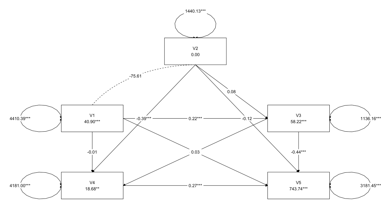
1 2 3 4 5 6 7 8 9 10 11 12 13 14 15 16 17 18 19 20 21 22 23 24 25 26 27 28 29 30 31 32 33 model1 <- ' # 因果关系 V3 ~ V1 + V2 V4 ~ V1 + V2 + V3 V5 ~ V1 + V2 + V3 + V4 # 协方差 V1 ~~ V2 # 指定残差 V3 ~~ V3 V4 ~~ V4 V5 ~~ V5 # 显式请求截距 V3 ~1 V4 ~1 V5 ~1 ' fit1 <- sem( model1, data= data) summary( fit1, fit.measures= TRUE , standardized= TRUE ) layout_matrix <- matrix( NA , nrow = 3 , ncol = 3 , dimnames = list ( NULL , NULL ) ) layout_matrix[ 1 , 2 ] <- "V2" layout_matrix[ 2 , 1 ] <- "V1" layout_matrix[ 2 , 3 ] <- "V3" layout_matrix[ 3 , 1 ] <- "V4" layout_matrix[ 3 , 3 ] <- "V5" graph_sem( fit1, layout = layout_matrix, text_size = 5 )
模型拟合结果
1 2 3 4 5 6 7 8 9 10 11 12 13 14 15 16 17 18 19 20 21 22 23 24 25 26 27 28 29 30 31 32 33 34 35 36 Model Test User Model: Test statistic 0.000 Degrees of freedom 0 Model Test Baseline Model: Test statistic 165.893 Degrees of freedom 10 P- value 0.000 User Model versus Baseline Model: Comparative Fit Index ( CFI) 1.000 Tucker- Lewis Index ( TLI) 1.000 Loglikelihood and Information Criteria: Loglikelihood user model ( H0) - 9938.865 Loglikelihood unrestricted model ( H1) - 9938.865 Akaike ( AIC) 19907.729 Bayesian ( BIC) 19966.553 Sample- size adjusted Bayesian ( SABIC) 19918.962 Root Mean Square Error of Approximation: RMSEA 0.000 90 Percent confidence interval - lower 0.000 90 Percent confidence interval - upper 0.000 P- value H_0: RMSEA <= 0.050 NA P- value H_0: RMSEA >= 0.080 NA Standardized Root Mean Square Residual: SRMR 0.000
参数估计结果与标准化参数估计结果
1 2 3 4 5 6 7 8 9 10 11 12 13 14 15 16 17 18 19 20 21 22 23 24 25 26 27 28 29 30 31 32 33 34 35 Regressions: Estimate Std.Err z- value P( > | z| ) Std.lv Std.all V3 ~ V1 0.217 0.026 8.260 0.000 0.217 0.392 V2 0.079 0.046 1.721 0.085 0.079 0.082 V4 ~ V1 - 0.014 0.055 - 0.261 0.794 - 0.014 - 0.014 V2 - 0.393 0.089 - 4.433 0.000 - 0.393 - 0.223 V3 - 0.198 0.099 - 1.995 0.046 - 0.198 - 0.109 V5 ~ V1 0.032 0.048 0.663 0.507 0.032 0.034 V2 - 0.122 0.079 - 1.533 0.125 - 0.122 - 0.074 V3 - 0.442 0.087 - 5.071 0.000 - 0.442 - 0.260 V4 0.271 0.045 6.005 0.000 0.271 0.291 Covariances: Estimate Std.Err z- value P( > | z| ) Std.lv Std.all V1 ~ ~ V2 - 75.607 130.551 - 0.579 0.562 - 75.607 - 0.030 Intercepts: Estimate Std.Err z- value P( > | z| ) Std.lv Std.all .V3 58.217 2.050 28.399 0.000 58.217 1.584 .V4 18.685 6.993 2.672 0.008 18.685 0.279 .V5 743.742 6.158 120.772 0.000 743.742 11.916 V1 40.900 3.439 11.894 0.000 40.900 0.616 V2 0.000 1.965 0.000 1.000 0.000 0.000 Variances: Estimate Std.Err z- value P( > | z| ) Std.lv Std.all .V3 1136.158 83.195 13.657 0.000 1136.158 0.841 .V4 4181.001 306.155 13.657 0.000 4181.001 0.934 .V5 3181.454 232.963 13.657 0.000 3181.454 0.817 V1 4410.394 322.952 13.657 0.000 4410.394 1.000 V2 1440.129 105.454 13.657 0.000 1440.129 1.000
可以看出V1 ~ V4、V2 ~ V3、V1 ~ V5、V2 ~ V5路径不显著,可以考虑后续模型修正。
间接因果效应计算
1 2 3 4 5 6 7 8 9 10 11 12 13 14 15 16 17 18 19 20 21 22 23 24 25 26 27 28 29 30 31 32 33 34 35 36 37 38 39 40 41 42 43 44 45 46 47 48 model2 <- ' # 因果关系 V3 ~ c1*V1 + c2*V2 V4 ~ b1*V1 + b2*V2 + b3*V3 V5 ~ a1*V1 + a2*V2 + a3*V3 + a4*V4 # 协方差 V1 ~~ V2 # 指定残差 V3 ~~ e3*V3 V4 ~~ e4*V4 V5 ~~ e5*V5 # 显式请求截距 V3 ~1 V4 ~1 V5 ~1 # 计算间接效应 # 间接效应: V1到V4通过V3 ind_V1_V4 := c1 * b3 # 间接效应: V1到V5通过V3和V4 ind_V1_V5 := a4 * (ind_V1_V4 + b1) + a3 * c1 # 间接效应: V2到V4通过V3 ind_V2_V4 := c2 * b3 # 间接效应: V2到V5通过V3和V4 ind_V2_V5 := a4 * (ind_V2_V4 + b2) + a3 * c2 # 间接效应: V3到V5通过V4 ind_V3_V5 := b3 * a4 # 计算总效应 # 总效应: V1到V4 total_V1_V4 := b1 + ind_V1_V4 # 总效应: V1到V5 total_V1_V5 := a1 + ind_V1_V5 # 总效应: V2到V4 total_V2_V4 := b2 + ind_V2_V4 # 总效应: V2到V5 total_V2_V5 := a2 + ind_V2_V5 # 总效应: V3到V5 total_V3_V5 := a3 + ind_V3_V5 ' fit2 <- sem( model2, data= data) summary( fit2, fit.measures= TRUE , standardized= TRUE )
间接效应与直接效应的估计值与标准化估计值
1 2 3 4 5 6 7 8 9 10 11 12 Defined Parameters: Estimate Std.Err z- value P( > | z| ) Std.lv Std.all ind_V1_V4 - 0.043 0.022 - 1.939 0.052 - 0.043 - 0.043 ind_V1_V5 - 0.112 0.027 - 4.181 0.000 - 0.112 - 0.119 ind_V2_V4 - 0.016 0.012 - 1.303 0.192 - 0.016 - 0.009 ind_V2_V5 - 0.146 0.038 - 3.822 0.000 - 0.146 - 0.089 ind_V3_V5 - 0.054 0.028 - 1.893 0.058 - 0.054 - 0.032 total_V1_V4 - 0.057 0.051 - 1.132 0.258 - 0.057 - 0.057 total_V1_V5 - 0.080 0.048 - 1.666 0.096 - 0.080 - 0.085 total_V2_V4 - 0.409 0.089 - 4.604 0.000 - 0.409 - 0.232 total_V2_V5 - 0.267 0.084 - 3.191 0.001 - 0.267 - 0.163 total_V3_V5 - 0.496 0.091 - 5.461 0.000 - 0.496 - 0.292
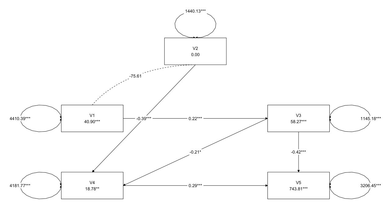
非饱和的递归模型
删去V2到V3路径以及V1到V4路径
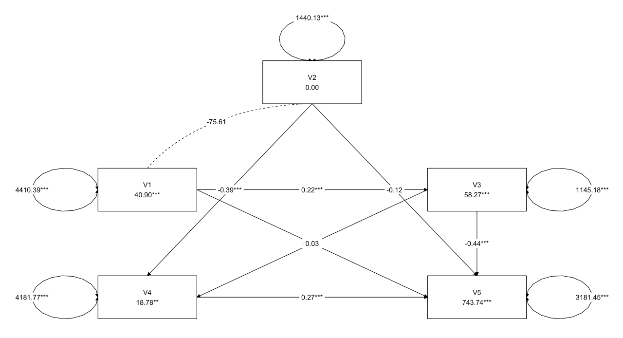
1 2 3 4 5 6 7 8 9 10 11 12 13 14 15 16 17 18 19 20 21 22 23 24 25 26 27 28 29 30 31 32 33 34 35 36 37 38 39 40 41 42 43 44 45 46 47 48 49 50 model3 <- ' # 因果关系 V3 ~ c1*V1 V4 ~ b2*V2 + b3*V3 V5 ~ a1*V1 + a2*V2 + a3*V3 + a4*V4 # 协方差 V1 ~~ V2 # 指定残差 V3 ~~ e3*V3 V4 ~~ e4*V4 V5 ~~ e5*V5 # 显式请求截距 V3 ~1 V4 ~1 V5 ~1 # 计算间接效应 # 间接效应: V1到V4通过V3 ind_V1_V4 := c1 * b3 # 间接效应: V1到V5通过V3和V4 ind_V1_V5 := c1 * b3 * a4 + c1 * a3 # 间接效应: V2到V5通过V4 ind_V2_V5 := b2 * a4 # 间接效应: V3到V5通过V4 ind_V3_V5 := b3 * a4 # 计算总效应 # 总效应: V1到V5 total_V1_V5 := a1 + ind_V1_V5 # 总效应: V2到V5 total_V2_V5 := a2 + ind_V2_V5 # 总效应: V3到V5 total_V3_V5 := a3 + ind_V3_V5 ' fit3 <- sem( model3, data= data) summary( fit3, fit.measures= TRUE , standardized= TRUE , estimates= TRUE ) layout_matrix <- matrix( NA , nrow = 3 , ncol = 3 , dimnames = list ( NULL , NULL ) ) layout_matrix[ 1 , 2 ] <- "V2" layout_matrix[ 2 , 1 ] <- "V1" layout_matrix[ 2 , 3 ] <- "V3" layout_matrix[ 3 , 1 ] <- "V4" layout_matrix[ 3 , 3 ] <- "V5" graph_sem( fit3, layout = layout_matrix, text_size = 5 )
模型拟合结果
1 2 3 4 5 6 7 8 9 10 11 12 13 14 15 16 17 18 19 20 21 22 23 24 25 26 27 28 29 30 31 32 33 34 35 36 37 Model Test User Model: Test statistic 3.019 Degrees of freedom 2 P- value ( Chi- square) 0.221 Model Test Baseline Model: Test statistic 165.893 Degrees of freedom 10 P- value 0.000 User Model versus Baseline Model: Comparative Fit Index ( CFI) 0.993 Tucker- Lewis Index ( TLI) 0.967 Loglikelihood and Information Criteria: Loglikelihood user model ( H0) - 9940.374 Loglikelihood unrestricted model ( H1) - 9938.865 Akaike ( AIC) 19916.748 Bayesian ( BIC) 19987.337 Sample- size adjusted Bayesian ( SABIC) 19930.228 Root Mean Square Error of Approximation: RMSEA 0.037 90 Percent confidence interval - lower 0.000 90 Percent confidence interval - upper 0.116 P- value H_0: RMSEA <= 0.050 0.493 P- value H_0: RMSEA >= 0.080 0.237 Standardized Root Mean Square Residual: SRMR 0.020
参数估计结果与标准化参数估计结果
1 2 3 4 5 6 7 8 9 10 11 12 13 14 15 16 17 18 19 20 21 22 23 24 25 26 27 28 29 30 31 32 33 34 35 36 37 38 39 40 41 42 43 Regressions: Estimate Std.Err z- value P( > | z| ) Std.lv Std.all V3 ~ V1 ( c1) 0.216 0.026 8.180 0.000 0.216 0.390 V4 ~ V2 ( b2) - 0.391 0.088 - 4.436 0.000 - 0.391 - 0.222 V3 ( b3) - 0.208 0.091 - 2.287 0.022 - 0.208 - 0.115 V5 ~ V1 ( a1) 0.032 0.048 0.664 0.507 0.032 0.034 V2 ( a2) - 0.122 0.079 - 1.539 0.124 - 0.122 - 0.074 V3 ( a3) - 0.442 0.087 - 5.088 0.000 - 0.442 - 0.261 V4 ( a4) 0.271 0.045 6.006 0.000 0.271 0.291 Covariances: Estimate Std.Err z- value P( > | z| ) Std.lv Std.all V1 ~ ~ V2 - 75.607 130.551 - 0.579 0.562 - 75.607 - 0.030 Intercepts: Estimate Std.Err z- value P( > | z| ) Std.lv Std.all .V3 58.273 2.058 28.318 0.000 58.273 1.586 .V4 18.783 6.971 2.695 0.007 18.783 0.281 .V5 743.742 6.146 121.004 0.000 743.742 11.954 V1 40.900 3.439 11.894 0.000 40.900 0.616 V2 0.000 1.965 0.000 1.000 0.000 0.000 Variances: Estimate Std.Err z- value P( > | z| ) Std.lv Std.all .V3 ( e3) 1145.182 83.856 13.657 0.000 1145.182 0.848 .V4 ( e4) 4181.767 306.211 13.657 0.000 4181.767 0.938 .V5 ( e5) 3181.453 232.963 13.657 0.000 3181.453 0.822 V1 4410.394 322.952 13.657 0.000 4410.394 1.000 V2 1440.129 105.454 13.657 0.000 1440.129 1.000 Defined Parameters: Estimate Std.Err z- value P( > | z| ) Std.lv Std.all ind_V1_V4 - 0.045 0.020 - 2.203 0.028 - 0.045 - 0.045 ind_V1_V5 - 0.108 0.023 - 4.593 0.000 - 0.108 - 0.115 ind_V2_V5 - 0.106 0.030 - 3.568 0.000 - 0.106 - 0.065 ind_V3_V5 - 0.057 0.026 - 2.137 0.033 - 0.057 - 0.033 total_V1_V5 - 0.076 0.046 - 1.640 0.101 - 0.076 - 0.081 total_V2_V5 - 0.228 0.081 - 2.824 0.005 - 0.228 - 0.139 total_V3_V5 - 0.498 0.090 - 5.550 0.000 - 0.498 - 0.294
可以看出V1 ~ V5、V2 ~ V5路径不显著,可以考虑后续模型修正。
1 2 3 4 5 6 7 > anova( fit2, fit3) Chi- Squared Difference Test Df AIC BIC Chisq Chisq diff RMSEA Df diff Pr( > Chisq) fit2 0 19918 19996 0.000 fit3 2 19917 19987 3.019 3.0189 0.036958 2 0.221
非饱和模型的卡方值Chisq为3.019,p值Pr(>Chisq)为0.221,即在0.05水平上不显著
但是RMSEA、CFI、TLI都达到了模型良好拟合的判断标准,而且相比饱和模型的拟合指数相比变化量更小,表明删去路径后非饱和模型能比饱和模型能够更好地拟合数据,统计上可以接受零假设,因此对原饱和模型进行修正,用该非饱和模型进行替代
删去V1到V5路径以及V2到V5路径
1 2 3 4 5 6 7 8 9 10 11 12 13 14 15 16 17 18 19 20 21 22 23 24 25 26 27 28 29 30 31 32 33 34 35 36 37 38 39 40 41 42 43 44 45 46 model4 <- ' # 因果关系 V3 ~ c1*V1 V4 ~ b2*V2 + b3*V3 V5 ~ a3*V3 + a4*V4 # 协方差 V1 ~~ V2 # 指定残差 V3 ~~ e3*V3 V4 ~~ e4*V4 V5 ~~ e5*V5 # 显式请求截距 V3 ~1 V4 ~1 V5 ~1 # 计算间接效应 # 间接效应: V1到V4通过V3 ind_V1_V4 := c1*b3 # 间接效应: V1到V5通过V3和V4 ind_V1_V5 := c1 * b3 * a4 + c1 * a3 # 间接效应: V2到V5通过V4 ind_V2_V5 := b2 * a4 # 间接效应: V3到V5通过V4 ind_V3_V5 := b3 * a4 # 计算总效应 # 总效应: V3到V5 total_V3_V5 := a3 + ind_V3_V5 ' fit4 <- sem( model4, data= data) summary( fit4, fit.measures= TRUE , standardized= TRUE , estimates= TRUE ) layout_matrix <- matrix( NA , nrow = 3 , ncol = 3 , dimnames = list ( NULL , NULL ) ) layout_matrix[ 1 , 2 ] <- "V2" layout_matrix[ 2 , 1 ] <- "V1" layout_matrix[ 2 , 3 ] <- "V3" layout_matrix[ 3 , 1 ] <- "V4" layout_matrix[ 3 , 3 ] <- "V5" graph_sem( fit4, layout = layout_matrix, text_size = 5 )
模型拟合结果
1 2 3 4 5 6 7 8 9 10 11 12 13 14 15 16 17 18 19 20 21 22 23 24 25 26 27 28 29 30 31 32 33 34 35 36 37 Model Test User Model: Test statistic 5.938 Degrees of freedom 4 P- value ( Chi- square) 0.204 Model Test Baseline Model: Test statistic 165.893 Degrees of freedom 10 P- value 0.000 User Model versus Baseline Model: Comparative Fit Index ( CFI) 0.988 Tucker- Lewis Index ( TLI) 0.969 Loglikelihood and Information Criteria: Loglikelihood user model ( H0) - 9941.834 Loglikelihood unrestricted model ( H1) - 9938.865 Akaike ( AIC) 19915.667 Bayesian ( BIC) 19978.412 Sample- size adjusted Bayesian ( SABIC) 19927.649 Root Mean Square Error of Approximation: RMSEA 0.036 90 Percent confidence interval - lower 0.000 90 Percent confidence interval - upper 0.092 P- value H_0: RMSEA <= 0.050 0.582 P- value H_0: RMSEA >= 0.080 0.113 Standardized Root Mean Square Residual: SRMR 0.029
参数估计结果与标准化参数估计结果
1 2 3 4 5 6 7 8 9 10 11 12 13 14 15 16 17 18 19 20 21 22 23 24 25 26 27 28 29 30 31 32 33 34 35 36 37 38 39 Regressions: Estimate Std.Err z- value P( > | z| ) Std.lv Std.all V3 ~ V1 ( c1) 0.216 0.026 8.180 0.000 0.216 0.390 V4 ~ V2 ( b2) - 0.391 0.088 - 4.436 0.000 - 0.391 - 0.222 V3 ( b3) - 0.208 0.091 - 2.287 0.022 - 0.208 - 0.115 V5 ~ V3 ( a3) - 0.424 0.080 - 5.287 0.000 - 0.424 - 0.250 V4 ( a4) 0.287 0.044 6.489 0.000 0.287 0.307 Covariances: Estimate Std.Err z- value P( > | z| ) Std.lv Std.all V1 ~ ~ V2 - 75.607 130.551 - 0.579 0.562 - 75.607 - 0.030 Intercepts: Estimate Std.Err z- value P( > | z| ) Std.lv Std.all .V3 58.273 2.058 28.318 0.000 58.273 1.586 .V4 18.783 6.971 2.695 0.007 18.783 0.281 .V5 743.808 6.158 120.790 0.000 743.808 11.936 V1 40.900 3.439 11.894 0.000 40.900 0.616 V2 0.000 1.965 0.000 1.000 0.000 0.000 Variances: Estimate Std.Err z- value P( > | z| ) Std.lv Std.all .V3 ( e3) 1145.182 83.856 13.657 0.000 1145.182 0.848 .V4 ( e4) 4181.767 306.211 13.657 0.000 4181.767 0.938 .V5 ( e5) 3206.449 234.793 13.657 0.000 3206.449 0.826 V1 4410.394 322.952 13.657 0.000 4410.394 1.000 V2 1440.129 105.454 13.657 0.000 1440.129 1.000 Defined Parameters: Estimate Std.Err z- value P( > | z| ) Std.lv Std.all ind_V1_V4 - 0.045 0.020 - 2.203 0.028 - 0.045 - 0.045 ind_V1_V5 - 0.105 0.022 - 4.714 0.000 - 0.105 - 0.111 ind_V2_V5 - 0.112 0.031 - 3.662 0.000 - 0.112 - 0.068 ind_V3_V5 - 0.060 0.028 - 2.157 0.031 - 0.060 - 0.035 total_V3_V5 - 0.484 0.084 - 5.768 0.000 - 0.484 - 0.286
1 2 3 4 5 6 7 8 > anova( fit2, fit3, fit4) Chi- Squared Difference Test Df AIC BIC Chisq Chisq diff RMSEA Df diff Pr( > Chisq) fit2 0 19918 19996 0.0000 fit3 2 19917 19987 3.0190 3.0189 0.036958 2 0.2210 fit4 4 19916 19978 5.9377 2.9188 0.035094 2 0.2324
结构方程模型
导入包与数据
1 2 3 4 5 6 7 8 9 10 11 library( lavaan) library( tidySEM) setwd( "/Users/nanxu/研究生课程作业/心理统计/课件数据/10第十章 结构方程模型/" ) data <- read.table( "./10_1.dat" , header = FALSE , sep = "" , na.strings = "NA" ) names ( data) dim ( data)
数据介绍
1 2 3 4 5 6 7 8 9 10 11 12 13 14 15 16 17 18 19 20 names ( data) <- c ( "work1" , "work2" , "ee1" , "ee2" , "ee3" , "dpl1" , "dpl2" , "pa1" , "pa2" , "pa3" , "Gender" ) data$ Gender <- factor( data$ Gender, levels = c ( 1 , 2 ) , labels = c ( "male" , "female" ) ) table( data$ Gender) summary( data)
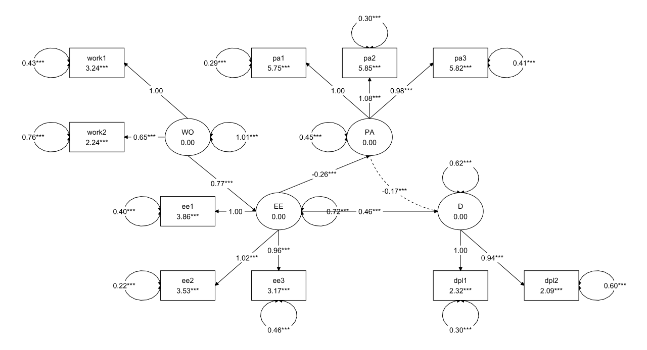
结构方程模型
1 2 3 4 5 6 7 8 9 10 11 12 13 14 15 16 17 18 19 20 21 22 23 24 25 26 27 28 29 30 31 32 33 34 35 36 37 38 39 40 41 42 43 44 45 46 47 48 49 50 model <- ' # 测量模型 EE =~ ee1 + ee2 + ee3 # EE 由 ee1, ee2, ee3 测量 D =~ dpl1 + dpl2 # D 由 dpl1, dpl2 测量 PA =~ pa1 + pa2 + pa3 # PA 由 pa1, pa2, pa3 测量 WO =~ work1 + work2 # WO 由 work1, work2 测量 # 结构模型 EE ~ WO # EE 被 WO 预测 D ~ EE # D 被 EE 预测 PA ~ EE # PA 被 EE 预测 # 协方差 PA ~~ D # PA 和 D 之间的协方差 # 截距 ee1 ~ 1 ee2 ~ 1 ee3 ~ 1 dpl1 ~ 1 dpl2 ~ 1 pa1 ~ 1 pa2 ~ 1 pa3 ~ 1 work1 ~ 1 work2 ~ 1 ' fit <- sem( model, data= data) summary( fit, fit.measures= TRUE , standardized= TRUE , rsquare= TRUE ) layout_matrix <- matrix( NA , nrow = 4 , ncol = 6 , dimnames = list ( NULL , NULL ) ) layout_matrix[ 1 , 1 ] <- "work1" layout_matrix[ 2 , 1 ] <- "work2" layout_matrix[ 2 , 2 ] <- "WO" layout_matrix[ 3 , 3 ] <- "EE" layout_matrix[ 3 , 2 ] <- "ee1" layout_matrix[ 4 , 2 ] <- "ee2" layout_matrix[ 4 , 3 ] <- "ee3" layout_matrix[ 2 , 4 ] <- "PA" layout_matrix[ 1 , 3 ] <- "pa1" layout_matrix[ 1 , 4 ] <- "pa2" layout_matrix[ 1 , 5 ] <- "pa3" layout_matrix[ 4 , 5 ] <- "dpl1" layout_matrix[ 4 , 6 ] <- "dpl2" layout_matrix[ 3 , 5 ] <- "D" graph_sem( fit, layout = layout_matrix, text_size = 5 )
模型拟合结果
1 2 3 4 5 6 7 8 9 10 11 12 13 14 15 16 17 18 19 20 21 22 23 24 25 26 27 28 29 30 31 32 33 34 35 36 37 Model Test User Model: Test statistic 301.492 Degrees of freedom 31 P- value ( Chi- square) 0.000 Model Test Baseline Model: Test statistic 7493.700 Degrees of freedom 45 P- value 0.000 User Model versus Baseline Model: Comparative Fit Index ( CFI) 0.964 Tucker- Lewis Index ( TLI) 0.947 Loglikelihood and Information Criteria: Loglikelihood user model ( H0) - 18293.991 Loglikelihood unrestricted model ( H1) - 18143.245 Akaike ( AIC) 36655.982 Bayesian ( BIC) 36835.006 Sample- size adjusted Bayesian ( SABIC) 36727.000 Root Mean Square Error of Approximation: RMSEA 0.078 90 Percent confidence interval - lower 0.070 90 Percent confidence interval - upper 0.086 P- value H_0: RMSEA <= 0.050 0.000 P- value H_0: RMSEA >= 0.080 0.360 Standardized Root Mean Square Residual: SRMR 0.040
可以看出,卡方值为301.492,自由度为31,CFI值为0.964,TLI值为0.947,RMSEA值为0.078,表明模型拟合较好。
模型估计结果
1 2 3 4 5 6 7 8 9 10 11 12 13 14 15 16 17 18 19 20 21 22 23 24 25 26 27 28 29 30 31 32 33 34 35 36 37 38 39 40 41 42 43 44 45 46 47 48 49 50 51 52 53 54 55 56 57 58 59 60 61 62 63 64 65 66 67 68 69 70 71 72 73 74 75 76 Latent Variables: Estimate Std.Err z- value P( > | z| ) Std.lv Std.all EE = ~ ee1 1.000 1.146 0.875 ee2 1.017 0.021 48.938 0.000 1.166 0.927 ee3 0.963 0.023 42.771 0.000 1.104 0.851 D = ~ dpl1 1.000 0.947 0.865 dpl2 0.941 0.044 21.591 0.000 0.891 0.754 PA = ~ pa1 1.000 0.738 0.809 pa2 1.076 0.036 29.617 0.000 0.794 0.825 pa3 0.979 0.035 27.854 0.000 0.723 0.750 WO = ~ work1 1.000 1.007 0.838 work2 0.652 0.039 16.585 0.000 0.656 0.602 Regressions: Estimate Std.Err z- value P( > | z| ) Std.lv Std.all EE ~ WO 0.766 0.046 16.490 0.000 0.673 0.673 D ~ EE 0.462 0.024 19.325 0.000 0.559 0.559 PA ~ EE - 0.262 0.019 - 13.776 0.000 - 0.408 - 0.408 Covariances: Estimate Std.Err z- value P( > | z| ) Std.lv Std.all .D ~ ~ .PA - 0.174 0.019 - 8.950 0.000 - 0.328 - 0.328 Intercepts: Estimate Std.Err z- value P( > | z| ) Std.lv Std.all .ee1 3.855 0.035 111.347 0.000 3.855 2.944 .ee2 3.530 0.033 106.201 0.000 3.530 2.808 .ee3 3.165 0.034 92.281 0.000 3.165 2.440 .dpl1 2.319 0.029 80.113 0.000 2.319 2.119 .dpl2 2.086 0.031 66.763 0.000 2.086 1.765 .pa1 5.748 0.024 238.172 0.000 5.748 6.298 .pa2 5.850 0.025 229.759 0.000 5.850 6.076 .pa3 5.815 0.025 228.188 0.000 5.815 6.034 .work1 3.240 0.032 101.996 0.000 3.240 2.697 .work2 2.243 0.029 77.885 0.000 2.243 2.060 Variances: Estimate Std.Err z- value P( > | z| ) Std.lv Std.all .ee1 0.400 0.021 19.017 0.000 0.400 0.234 .ee2 0.222 0.017 13.108 0.000 0.222 0.140 .ee3 0.463 0.022 20.743 0.000 0.463 0.275 .dpl1 0.302 0.037 8.137 0.000 0.302 0.252 .dpl2 0.603 0.039 15.621 0.000 0.603 0.432 .pa1 0.288 0.017 16.743 0.000 0.288 0.346 .pa2 0.296 0.019 15.573 0.000 0.296 0.320 .pa3 0.406 0.020 20.150 0.000 0.406 0.438 .work1 0.429 0.054 7.876 0.000 0.429 0.297 .work2 0.756 0.036 21.071 0.000 0.756 0.637 .EE 0.719 0.048 15.109 0.000 0.547 0.547 .D 0.616 0.044 14.058 0.000 0.687 0.687 .PA 0.454 0.028 16.485 0.000 0.834 0.834 WO 1.014 0.073 13.851 0.000 1.000 1.000 R- Square: Estimate ee1 0.766 ee2 0.860 ee3 0.725 dpl1 0.748 dpl2 0.568 pa1 0.654 pa2 0.680 pa3 0.562 work1 0.703 work2 0.363 EE 0.453 D 0.313 PA 0.166
结构方程模型多组比较
不同性别分别拟合模型
1 2 3 4 5 6 7 8 9 10 11 12 data_male <- subset( data, Gender == "male" ) data_female <- subset( data, Gender == "female" ) fit_male <- cfa( model, data = data_male) summary( fit_male, fit.measures = TRUE , standardized = TRUE , rsquare = TRUE ) fit_female <- cfa( model, data = data_female) summary( fit_female, fit.measures = TRUE , standardized = TRUE , rsquare = TRUE )
1 2 3 4 5 6 7 8 9 10 11 12 13 14 15 16 17 18 19 20 21 22 23 24 25 26 27 28 29 30 31 32 33 34 35 36 37 38 39 40 41 > summary( fit_male, fit.measures = TRUE , standardized = TRUE , rsquare = TRUE ) Model Test User Model: Test statistic 201.953 Degrees of freedom 31 P- value ( Chi- square) 0.000 User Model versus Baseline Model: Comparative Fit Index ( CFI) 0.954 Tucker- Lewis Index ( TLI) 0.933 Root Mean Square Error of Approximation: RMSEA 0.088 90 Percent confidence interval - lower 0.077 90 Percent confidence interval - upper 0.100 P- value H_0: RMSEA <= 0.050 0.000 P- value H_0: RMSEA >= 0.080 0.878 > summary( fit_female, fit.measures = TRUE , standardized = TRUE , rsquare = TRUE ) Model Test User Model: Test statistic 157.743 Degrees of freedom 31 P- value ( Chi- square) 0.000 User Model versus Baseline Model: Comparative Fit Index ( CFI) 0.967 Tucker- Lewis Index ( TLI) 0.951 Root Mean Square Error of Approximation: RMSEA 0.076 90 Percent confidence interval - lower 0.064 90 Percent confidence interval - upper 0.087 P- value H_0: RMSEA <= 0.050 0.000 P- value H_0: RMSEA >= 0.080 0.276
结构模式相同模型(基线模型)
1 2 3 fit_baseline <- sem( model, data = data, group = "Gender" ) summary( fit_baseline, fit.measures= TRUE , standardized= TRUE , rsquare= TRUE )
1 2 3 4 5 6 7 8 9 10 11 12 13 14 15 16 17 18 19 20 21 22 23 > summary( fit_baseline, fit.measures= TRUE , standardized= TRUE , rsquare= TRUE ) Model Test User Model: Test statistic 359.696 Degrees of freedom 62 P- value ( Chi- square) 0.000 Test statistic for each group: female 157.743 male 201.953 User Model versus Baseline Model: Comparative Fit Index ( CFI) 0.960 Tucker- Lewis Index ( TLI) 0.942 Root Mean Square Error of Approximation: RMSEA 0.082 90 Percent confidence interval - lower 0.074 90 Percent confidence interval - upper 0.090 P- value H_0: RMSEA <= 0.050 0.000 P- value H_0: RMSEA >= 0.080 0.662
可以看出RMSEA值为0.082,CFI的值为0.960,TLI的值为0.942,卡方值为359.696,自由度为62,表明模型拟合较好。该模型作为基线模型,用于检验其他等价性条件是否满足。
测量模型:因素载荷等价模型(弱等价性)
1 2 3 4 fit_metric <- update( fit_baseline, group.equal = "loadings" ) summary( fit_metric, fit.measures= TRUE , standardized= TRUE , rsquare= TRUE ) anova( fit_baseline, fit_metric)
1 2 3 4 5 6 7 > anova( fit_baseline, fit_metric) Chi- Squared Difference Test Df AIC BIC Chisq Chisq diff RMSEA Df diff Pr( > Chisq) fit_baseline 62 36683 37041 359.70 fit_metric 68 36675 37002 364.27 4.5749 0 6 0.5994
弱等价性模型嵌套于基线模型,可以使用嵌套模型的比较方法。
可以看出两个模型的卡方值的差值Chisq diff为4.5749,自由度的差值Df diff为6,表明两个模型的卡方差异不显著。可以接受弱等价模型,即认为不同性别之间满足因素载荷等价条件。
测量模型:误差协方差矩阵等价模型
1 2 3 4 fit_residuals <- update( fit_metric, group.equal = c ( "loadings" , "residuals" ) ) summary( fit_residuals, fit.measures= TRUE , standardized= TRUE , rsquare= TRUE ) anova( fit_baseline, fit_metric, fit_residuals)
1 2 3 4 5 6 7 8 > anova( fit_baseline, fit_metric, fit_residuals) Chi- Squared Difference Test Df AIC BIC Chisq Chisq diff RMSEA Df diff Pr( > Chisq) fit_baseline 62 36683 37041 359.70 fit_metric 68 36675 37002 364.27 4.5749 0.000000 6 0.5994 fit_residuals 78 36670 36944 379.52 15.2466 0.027089 10 0.1233
可以看出两个模型的卡方值的差值Chisq diff为15.2466,自由度的差值Df diff为10,表明两个模型的卡方差异不显著。可以接受误差方差等价模型,即认为不同性别之间满足误差方差等价条件。
测量模型:截距等价模型
1 2 3 fit_scalar <- update( fit_residuals, group.equal = c ( "loadings" , "residuals" , "intercepts" ) ) summary( fit_scalar, fit.measures= TRUE , standardized= TRUE , rsquare= TRUE ) anova( fit_baseline, fit_metric, fit_residuals, fit_scalar)
1 2 3 4 5 6 7 8 9 > anova( fit_baseline, fit_metric, fit_residuals, fit_scalar) Chi- Squared Difference Test Df AIC BIC Chisq Chisq diff RMSEA Df diff Pr( > Chisq) fit_baseline 62 36683 37041 359.70 fit_metric 68 36675 37002 364.27 4.5749 0.000000 6 0.5994 fit_residuals 78 36670 36944 379.52 15.2466 0.027089 10 0.1233 fit_scalar 84 36663 36905 384.07 4.5511 0.000000 6 0.6025
可以看出两个模型的卡方值的差值Chisq diff为4.5511,自由度的差值Df diff为6,表明两个模型的卡方差异不显著。可以接受强等价模型,即认为不同性别之间满足截距等价条件。
结构模型:潜变量路径系数等价模型
1 2 3 4 fit_structural <- update( fit_scalar, group.equal = c ( "loadings" , "residuals" , "intercepts" , "regressions" ) ) summary( fit_structural, fit.measures = TRUE , standardized = TRUE , rsquare = TRUE ) anova( fit_baseline, fit_metric, fit_residuals, fit_scalar, fit_structural)
1 2 3 4 5 6 7 8 9 10 > anova( fit_baseline, fit_metric, fit_residuals, fit_scalar, fit_structural) Chi- Squared Difference Test Df AIC BIC Chisq Chisq diff RMSEA Df diff Pr( > Chisq) fit_baseline 62 36683 37041 359.70 fit_metric 68 36675 37002 364.27 4.5749 0.000000 6 0.5994 fit_residuals 78 36670 36944 379.52 15.2466 0.027089 10 0.1233 fit_scalar 84 36663 36905 384.07 4.5511 0.000000 6 0.6025 fit_structural 87 36662 36889 389.60 5.5357 0.034382 3 0.1365
可以看出两个模型的卡方值的差值Chisq diff为5.5357,自由度的差值Df diff为4,表明两个模型的卡方差异不显著。可以接受潜变量路径系数等价模型,即认为不同性别之间满足路径系数等价条件。
结构模型:潜变量协方差矩阵等价模型
1 2 3 4 fit_covariance <- update( fit_structural, group.equal = c ( "loadings" , "residuals" , "intercepts" , "regressions" , "lv.covariances" ) ) summary( fit_covariance, fit.measures= TRUE , standardized= TRUE , rsquare= TRUE ) anova( fit_baseline, fit_metric, fit_residuals, fit_scalar, fit_structural, fit_covariance)
1 2 3 4 5 6 7 8 9 10 11 > anova( fit_baseline, fit_metric, fit_residuals, fit_scalar, fit_structural, fit_covariance) Chi- Squared Difference Test Df AIC BIC Chisq Chisq diff RMSEA Df diff Pr( > Chisq) fit_baseline 62 36683 37041 359.70 fit_metric 68 36675 37002 364.27 4.5749 0.000000 6 0.5994 fit_residuals 78 36670 36944 379.52 15.2466 0.027089 10 0.1233 fit_scalar 84 36663 36905 384.07 4.5511 0.000000 6 0.6025 fit_structural 87 36662 36889 389.60 5.5357 0.034382 3 0.1365 fit_covariance 88 36662 36883 391.08 1.4783 0.025865 1 0.2240
可以看出两个模型的卡方值的差值Chisq diff为1.4783,自由度的差值Df diff为1,表明两个模型的卡方差异不显著。可以接受潜变量协方差等价模型,即认为不同性别之间满足潜变量协方差等价条件。
结构模型:潜变量方差等价模型
1 2 3 4 fit_variances <- update( fit_covariance, group.equal = c ( "loadings" , "residuals" , "intercepts" , "regressions" , "lv.covariances" , "lv.variances" ) ) summary( fit_variances, fit.measures= TRUE , standardized= TRUE , rsquare= TRUE ) anova( fit_baseline, fit_metric, fit_residuals, fit_scalar, fit_covariance, fit_variances)
1 2 3 4 5 6 7 8 9 10 11 12 > anova( fit_baseline, fit_metric, fit_residuals, fit_scalar, fit_structural, fit_covariance, fit_variances) Chi- Squared Difference Test Df AIC BIC Chisq Chisq diff RMSEA Df diff Pr( > Chisq) fit_baseline 62 36683 37041 359.70 fit_metric 68 36675 37002 364.27 4.5749 0.000000 6 0.5994 fit_residuals 78 36670 36944 379.52 15.2466 0.027089 10 0.1233 fit_scalar 84 36663 36905 384.07 4.5511 0.000000 6 0.6025 fit_structural 87 36662 36889 389.60 5.5357 0.034382 3 0.1365 fit_covariance 88 36662 36883 391.08 1.4783 0.025865 1 0.2240 fit_variances 92 36660 36860 397.44 6.3575 0.028710 4 0.1740
可以看出两个模型的卡方值的差值Chisq diff为6.3575,自由度的差值Df diff为4,表明两个模型的卡方差异不显著。可以接受潜变量方差等价模型,即认为不同性别之间满足潜变量方差等价条件。
结构模型:潜在因素均值等价模型
1 2 3 4 fit_means <- update( fit_variances, group.equal = c ( "loadings" , "residuals" , "intercepts" , "regressions" , "lv.covariances" , "lv.variances" , "means" ) ) summary( fit_means, fit.measures= TRUE , standardized= TRUE , rsquare= TRUE ) anova( fit_baseline, fit_metric, fit_residuals, fit_scalar, fit_covariance, fit_means)
1 2 3 4 5 6 7 8 9 10 11 12 13 > anova( fit_baseline, fit_metric, fit_residuals, fit_scalar, fit_structural, fit_covariance, fit_variances, fit_means) Chi- Squared Difference Test Df AIC BIC Chisq Chisq diff RMSEA Df diff Pr( > Chisq) fit_baseline 62 36683 37041 359.70 fit_metric 68 36675 37002 364.27 4.5749 0.000000 6 0.5994 fit_residuals 78 36670 36944 379.52 15.2466 0.027089 10 0.1233 fit_scalar 84 36663 36905 384.07 4.5511 0.000000 6 0.6025 fit_structural 87 36662 36889 389.60 5.5357 0.034382 3 0.1365 fit_covariance 88 36662 36883 391.08 1.4783 0.025865 1 0.2240 fit_variances 92 36660 36860 397.44 6.3575 0.028710 4 0.1740 fit_means 96 36656 36835 401.14 3.6989 0.000000 4 0.4483
可以看出两个模型的卡方值的差值Chisq diff为3.6989,自由度的差值Df diff为4,表明两个模型的卡方差异不显著。可以接受潜变量均值等价模型,即认为不同性别之间满足潜变量均值等价条件。
中介分析
导入包与数据
1 2 3 4 5 6 7 8 9 10 11 12 library( lavaan) library( tidySEM) library( blavaan) setwd( "/Users/nanxu/研究生课程作业/心理统计/课件数据/11第十一章 中介分析/" ) data <- read.table( "./11_4 med.dat" , header = FALSE , sep = "" , na.strings = "NA" ) names ( data) dim ( data)
数据介绍
1 2 3 4 5 6 7 8 9 10 11 12 13 14 15 16 17 18 19 20 21 22 23 24 25 26 27 28 29 30 names ( data) <- c ( "ID" , "nrel1" , "nrel2" , "nrel3" , "prel1" , "prel2" , "prel3" , "pem1" , "pem2" , "pem3" , "nem1" , "nem2" , "nem3" , "sat1" , "sat2" , "sat3" , "nrel_m" , "prel_m" , "pem_m" , "nem_m" , "sat_m" ) summary( data)
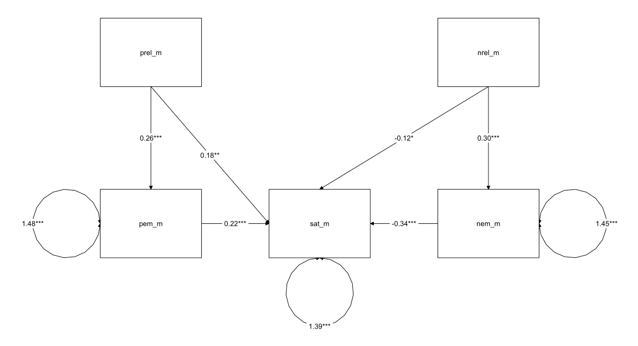
中介分析模型
1 2 3 4 5 6 7 8 9 10 11 12 13 14 15 16 17 18 19 20 21 22 23 24 med_model <- ' # 直接效应 sat_m ~ a1*pem_m + a2*nem_m + a3*prel_m + a4*nrel_m pem_m ~ b*prel_m nem_m ~ c*nrel_m # 计算间接效应(使用正确的参数定义方式) # 间接效应: sat_m 对 pem_m 通过 prel_m ind_pem_sat := b * a1 # 间接效应: sat_m 对 nem_m 通过 nrel_m ind_nem_sat := c * a2 ' fit <- sem( med_model, data= data) layout_matrix <- matrix( NA , nrow = 2 , ncol = 3 , dimnames = list ( NULL , NULL ) ) layout_matrix[ 1 , 1 ] <- "prel_m" layout_matrix[ 1 , 3 ] <- "nrel_m" layout_matrix[ 2 , 1 ] <- "pem_m" layout_matrix[ 2 , 2 ] <- "sat_m" layout_matrix[ 2 , 3 ] <- "nem_m" graph_sem( fit, layout = layout_matrix, text_size = 5 )
Sobel检验
1 2 fit1 <- sem( med_model, data= data) summary( fit1, fit.measures= TRUE , standardized= TRUE , rsquare= TRUE )
模型拟合结果
1 2 3 4 5 6 7 8 9 10 11 12 13 14 15 16 17 18 19 20 21 22 23 24 25 26 27 28 29 30 31 32 33 34 35 36 37 Model Test User Model: Test statistic 2.804 Degrees of freedom 3 P- value ( Chi- square) 0.423 Model Test Baseline Model: Test statistic 109.942 Degrees of freedom 9 P- value 0.000 User Model versus Baseline Model: Comparative Fit Index ( CFI) 1.000 Tucker- Lewis Index ( TLI) 1.006 Loglikelihood and Information Criteria: Loglikelihood user model ( H0) - 1249.213 Loglikelihood unrestricted model ( H1) - 1247.811 Akaike ( AIC) 2516.426 Bayesian ( BIC) 2548.472 Sample- size adjusted Bayesian ( SABIC) 2519.938 Root Mean Square Error of Approximation: RMSEA 0.000 90 Percent confidence interval - lower 0.000 90 Percent confidence interval - upper 0.102 P- value H_0: RMSEA <= 0.050 0.664 P- value H_0: RMSEA >= 0.080 0.135 Standardized Root Mean Square Residual: SRMR 0.025
可以看出,卡方值为2.804,自由度为3,CFI值为1.000,TLI值为1.006,RMSEA值为0.000,表明模型拟合较好。
参数估计结果与标准化参数估计结果
1 2 3 4 5 6 7 8 9 10 11 12 13 14 15 16 17 18 19 20 21 22 23 Regressions: Estimate Std.Err z- value P( > | z| ) Std.lv Std.all sat_m ~ pem_m ( a1) 0.219 0.060 3.654 0.000 0.219 0.206 nem_m ( a2) - 0.335 0.061 - 5.543 0.000 - 0.335 - 0.317 prel_m ( a3) 0.184 0.062 2.972 0.003 0.184 0.168 nrel_m ( a4) - 0.121 0.062 - 1.966 0.049 - 0.121 - 0.112 pem_m ~ prel_m ( b) 0.256 0.062 4.140 0.000 0.256 0.249 nem_m ~ nrel_m ( c ) 0.297 0.061 4.907 0.000 0.297 0.291 Variances: Estimate Std.Err z- value P( > | z| ) Std.lv Std.all .sat_m 1.385 0.121 11.402 0.000 1.385 0.778 .pem_m 1.484 0.130 11.402 0.000 1.484 0.938 .nem_m 1.455 0.128 11.402 0.000 1.455 0.915 R- Square: Estimate sat_m 0.222 pem_m 0.062 nem_m 0.085
中介效应检验结果
1 2 3 4 Defined Parameters: Estimate Std.Err z- value P( > | z| ) Std.lv Std.all ind_pem_sat 0.056 0.020 2.739 0.006 0.056 0.051 ind_nem_sat - 0.100 0.027 - 3.674 0.000 - 0.100 - 0.092
两个中介效应结果显著。
Bootstrap检验
1 2 3 4 5 6 7 8 9 10 fit2 <- sem( med_model, data= data, se= "bootstrap" , bootstrap= 1000 ) summary( fit2, fit.measures= TRUE , standardized= TRUE , rsquare= TRUE ) parameterEstimates( fit2, level= 0.90 , boot.ci.type= "bca" ) parameterEstimates( fit2, level= 0.95 , boot.ci.type= "bca" ) parameterEstimates( fit2, level= 0.99 , boot.ci.type= "bca" )
结果呈现了估计值est、90%置信区间、95%置信区间、99%置信区间
1 2 3 4 5 6 7 8 9 10 11 12 13 14 > parameterEstimates( fit2, level= 0.90 , boot.ci.type= "bca" ) lhs op rhs label est se z pvalue ci.lower ci.upper 13 ind_pem_sat := b* a1 ind_pem_sat 0.056 0.020 2.803 0.005 0.029 0.096 14 ind_nem_sat := c * a2 ind_nem_sat - 0.100 0.027 - 3.733 0.000 - 0.148 - 0.061 > parameterEstimates( fit2, level= 0.95 , boot.ci.type= "bca" ) lhs op rhs label est se z pvalue ci.lower ci.upper 13 ind_pem_sat := b* a1 ind_pem_sat 0.056 0.020 2.803 0.005 0.024 0.103 14 ind_nem_sat := c * a2 ind_nem_sat - 0.100 0.027 - 3.733 0.000 - 0.158 - 0.054 > parameterEstimates( fit2, level= 0.99 , boot.ci.type= "bca" ) lhs op rhs label est se z pvalue ci.lower ci.upper 13 ind_pem_sat := b* a1 ind_pem_sat 0.056 0.020 2.803 0.005 0.016 0.118 14 ind_nem_sat := c * a2 ind_nem_sat - 0.100 0.027 - 3.733 0.000 - 0.183 - 0.044
两个中介效应的置信区间均不包括0,说明两个中介效应均在0.10、0.05、0.01水平上显著
MCMC方法
1 2 3 4 5 6 7 8 9 10 fit3 <- bsem( med_model, data = data, n.chains = 2 , burnin = 1000 , sample = 30000 , adapt = 1000 , target = "stan" , seed = 12345 , save.lvs = FALSE ) summary( fit3)
1 2 3 4 5 6 7 8 9 10 11 12 13 14 15 16 17 18 19 20 21 22 Regressions: Estimate Post.SD pi.lower pi.upper Rhat Prior sat_m ~ pem_m ( a1) 0.219 0.061 0.101 0.337 1.000 normal( 0 , 10 ) nem_m ( a2) - 0.335 0.061 - 0.455 - 0.215 1.000 normal( 0 , 10 ) prel_m ( a3) 0.184 0.063 0.060 0.307 1.000 normal( 0 , 10 ) nrel_m ( a4) - 0.121 0.063 - 0.245 0.002 1.000 normal( 0 , 10 ) pem_m ~ prel_m ( b) 0.257 0.062 0.135 0.378 1.000 normal( 0 , 10 ) nem_m ~ nrel_m ( c ) 0.297 0.061 0.177 0.415 1.000 normal( 0 , 10 ) Variances: Estimate Post.SD pi.lower pi.upper Rhat Prior .sat_m 1.420 0.126 1.194 1.689 1.000 gamma ( 1 , .5 ) [ sd] .pem_m 1.503 0.134 1.264 1.791 1.000 gamma ( 1 , .5 ) [ sd] .nem_m 1.474 0.132 1.238 1.754 1.000 gamma ( 1 , .5 ) [ sd] Defined Parameters: Estimate Post.SD pi.lower pi.upper Rhat Prior ind_pem_sat 0.056 0.021 0.015 0.097 ind_nem_sat - 0.099 0.028 - 0.154 - 0.045
可以看出ind_pem_sat中介效应的95%置信区间估计为[0.015, 0.097],ind_nem_sat中介效应的95%置信区间估计为[-0.154, -0.045]
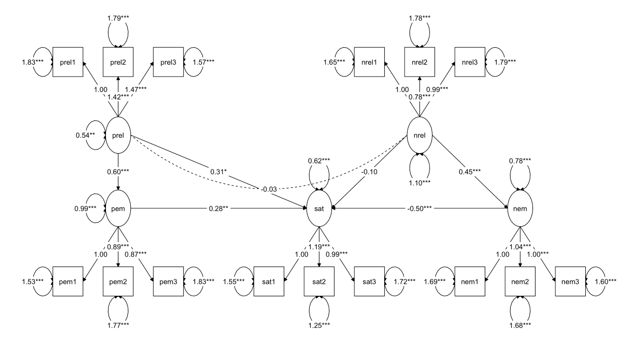
潜变量中介分析
1 2 3 4 5 6 7 8 9 10 11 12 13 14 15 16 17 18 19 20 21 22 23 24 25 26 27 28 29 30 31 32 33 34 35 36 37 38 39 40 41 42 43 44 45 46 47 48 med_latent_model <- ' # 测量模型 nrel =~ nrel1 + nrel2 + nrel3 prel =~ prel1 + prel2 + prel3 nem =~ nem1 + nem2 + nem3 pem =~ pem1 + pem2 + pem3 sat =~ sat1 + sat2 + sat3 # 结构模型 sat ~ a1*pem + a2*nem + a3*prel + a4*nrel pem ~ b*prel nem ~ c*nrel # 间接效应 # sat 对 pem 通过 prel sat_prel_prel := b * a1 # sat 对 nem 通过 nrel sat_nrel_nrel := c * a2 ' fit3 <- sem( med_latent_model, data= data) summary( fit3, fit.measures= TRUE , standardized= TRUE , rsquare= TRUE ) layout_matrix <- matrix( NA , nrow = 4 , ncol = 11 , dimnames = list ( NULL , NULL ) ) layout_matrix[ 1 , 1 ] <- "prel1" layout_matrix[ 1 , 2 ] <- "prel2" layout_matrix[ 1 , 3 ] <- "prel3" layout_matrix[ 2 , 2 ] <- "prel" layout_matrix[ 1 , 7 ] <- "nrel1" layout_matrix[ 1 , 8 ] <- "nrel2" layout_matrix[ 1 , 9 ] <- "nrel3" layout_matrix[ 2 , 8 ] <- "nrel" layout_matrix[ 4 , 1 ] <- "pem1" layout_matrix[ 4 , 2 ] <- "pem2" layout_matrix[ 4 , 3 ] <- "pem3" layout_matrix[ 3 , 2 ] <- "pem" layout_matrix[ 4 , 5 ] <- "sat1" layout_matrix[ 4 , 6 ] <- "sat2" layout_matrix[ 4 , 7 ] <- "sat3" layout_matrix[ 3 , 6 ] <- "sat" layout_matrix[ 4 , 9 ] <- "nem1" layout_matrix[ 4 , 10 ] <- "nem2" layout_matrix[ 4 , 11 ] <- "nem3" layout_matrix[ 3 , 10 ] <- "nem" graph_sem( fit3, layout = layout_matrix, text_size = 5 )
模型拟合结果
1 2 3 4 5 6 7 8 9 10 11 12 13 14 15 16 17 18 19 20 21 22 23 24 25 26 27 28 29 30 31 32 33 34 35 36 37 Model Test User Model: Test statistic 80.049 Degrees of freedom 83 P- value ( Chi- square) 0.571 Model Test Baseline Model: Test statistic 714.854 Degrees of freedom 105 P- value 0.000 User Model versus Baseline Model: Comparative Fit Index ( CFI) 1.000 Tucker- Lewis Index ( TLI) 1.006 Loglikelihood and Information Criteria: Loglikelihood user model ( H0) - 7162.602 Loglikelihood unrestricted model ( H1) - 7122.577 Akaike ( AIC) 14399.204 Bayesian ( BIC) 14530.950 Sample- size adjusted Bayesian ( SABIC) 14413.645 Root Mean Square Error of Approximation: RMSEA 0.000 90 Percent confidence interval - lower 0.000 90 Percent confidence interval - upper 0.032 P- value H_0: RMSEA <= 0.050 1.000 P- value H_0: RMSEA >= 0.080 0.000 Standardized Root Mean Square Residual: SRMR 0.043
参数估计结果与标准化参数估计结果
1 2 3 4 5 6 7 8 9 10 11 12 13 14 15 16 17 18 19 20 21 22 23 24 25 26 27 28 29 30 31 32 33 34 35 36 37 38 39 40 41 42 43 44 45 46 47 48 49 50 51 52 53 54 55 56 57 58 59 60 61 62 63 64 65 66 67 68 69 70 71 72 73 74 75 76 77 78 79 80 81 82 83 Latent Variables: Estimate Std.Err z- value P( > | z| ) Std.lv Std.all nrel = ~ nrel1 1.000 1.051 0.633 nrel2 0.782 0.147 5.334 0.000 0.822 0.524 nrel3 0.989 0.179 5.515 0.000 1.039 0.614 prel = ~ prel1 1.000 0.736 0.478 prel2 1.422 0.282 5.047 0.000 1.047 0.616 prel3 1.471 0.293 5.022 0.000 1.083 0.654 nem = ~ nem1 1.000 1.004 0.612 nem2 1.045 0.163 6.422 0.000 1.048 0.628 nem3 1.000 0.156 6.399 0.000 1.003 0.621 pem = ~ pem1 1.000 1.090 0.661 pem2 0.894 0.153 5.852 0.000 0.975 0.591 pem3 0.869 0.150 5.809 0.000 0.948 0.573 sat = ~ sat1 1.000 1.065 0.650 sat2 1.189 0.148 8.059 0.000 1.266 0.750 sat3 0.994 0.132 7.557 0.000 1.058 0.627 Regressions: Estimate Std.Err z- value P( > | z| ) Std.lv Std.all sat ~ pem ( a1) 0.278 0.099 2.806 0.005 0.285 0.285 nem ( a2) - 0.498 0.126 - 3.963 0.000 - 0.469 - 0.469 prel ( a3) 0.310 0.147 2.108 0.035 0.215 0.215 nrel ( a4) - 0.096 0.105 - 0.912 0.362 - 0.095 - 0.095 pem ~ prel ( b) 0.599 0.174 3.440 0.001 0.404 0.404 nem ~ nrel ( c ) 0.449 0.112 4.017 0.000 0.470 0.470 Covariances: Estimate Std.Err z- value P( > | z| ) Std.lv Std.all nrel ~ ~ prel - 0.034 0.075 - 0.457 0.648 - 0.044 - 0.044 Variances: Estimate Std.Err z- value P( > | z| ) Std.lv Std.all .nrel1 1.653 0.237 6.965 0.000 1.653 0.599 .nrel2 1.779 0.199 8.939 0.000 1.779 0.725 .nrel3 1.787 0.243 7.366 0.000 1.787 0.623 .prel1 1.828 0.193 9.469 0.000 1.828 0.771 .prel2 1.793 0.251 7.151 0.000 1.793 0.621 .prel3 1.570 0.248 6.326 0.000 1.570 0.572 .nem1 1.686 0.204 8.265 0.000 1.686 0.626 .nem2 1.685 0.211 7.971 0.000 1.685 0.605 .nem3 1.602 0.198 8.099 0.000 1.602 0.614 .pem1 1.532 0.228 6.709 0.000 1.532 0.563 .pem2 1.773 0.218 8.130 0.000 1.773 0.651 .pem3 1.835 0.218 8.434 0.000 1.835 0.671 .sat1 1.549 0.181 8.542 0.000 1.549 0.577 .sat2 1.247 0.193 6.456 0.000 1.247 0.437 .sat3 1.724 0.194 8.888 0.000 1.724 0.606 nrel 1.105 0.270 4.094 0.000 1.000 1.000 prel 0.542 0.171 3.179 0.001 1.000 1.000 .nem 0.784 0.195 4.014 0.000 0.779 0.779 .pem 0.994 0.241 4.124 0.000 0.837 0.837 .sat 0.616 0.149 4.141 0.000 0.543 0.543 R- Square: Estimate nrel1 0.401 nrel2 0.275 nrel3 0.377 prel1 0.229 prel2 0.379 prel3 0.428 nem1 0.374 nem2 0.395 nem3 0.386 pem1 0.437 pem2 0.349 pem3 0.329 sat1 0.423 sat2 0.563 sat3 0.394 nem 0.221 pem 0.163 sat 0.457
Sobel检验
1 2 3 4 Defined Parameters: Estimate Std.Err z- value P( > | z| ) Std.lv Std.all sat_prel_sat 0.167 0.071 2.348 0.019 0.115 0.115 sat_nrel_sat - 0.224 0.073 - 3.054 0.002 - 0.221 - 0.221
结果显示,两个中介效应均显著
调节效应
两个连续变量的调节作用
自变量X X X M M M Y Y Y
导入包与数据
1 2 3 4 5 6 7 8 9 10 11 12 library( haven) library( lavaan) library( dplyr) setwd( "/Users/nanxu/研究生课程作业/心理统计/课件数据/12第十二章 调节效应/" ) data <- read_sav( "./12_1 mod_1.sav" ) names ( data) dim ( data)
数据介绍与预处理
1 2 3 4 5 6 summary( data) cor_matrix <- cor( data[ , 1 : 3 ] , use= "complete.obs" ) cor.plot( cor_matrix)
1 2 3 4 5 6 7 8 9 10 11 12 data$ CSC <- scale( data$ SC, scale = FALSE ) [ , 1 ] data$ CSS <- scale( data$ SS, scale = FALSE ) [ , 1 ] data$ ZSC <- scale( data$ SC) [ , 1 ] data$ ZSS <- scale( data$ SS) [ , 1 ] data$ ZDEP <- scale( data$ DEP) [ , 1 ] data$ CSSCSC <- data$ CSC * data$ CSS data$ ZSSZSC <- data$ ZSC * data$ ZSS
非标准化解
将自变量X X X M M M
1 2 3 4 5 6 7 8 9 10 fit1 <- lm( DEP ~ CSS + CSC, data = data) summary( fit1) fit2 <- lm( DEP ~ CSS + CSC + CSSCSC, data = data) summary( fit2) anova( fit1, fit2)
回归系数估计结果
1 2 3 4 5 6 7 8 9 10 11 12 13 14 15 16 17 18 19 20 21 22 23 24 25 26 27 28 > summary( fit1) Coefficients: Estimate Std. Error t value Pr( > | t| ) ( Intercept) 2.55711 0.05698 44.874 < 2e-16 * * * CSS 0.30851 0.09203 3.352 0.000937 * * * CSC - 0.23512 0.11750 - 2.001 0.046571 * - - - Signif. codes: 0 ‘* * * ’ 0.001 ‘* * ’ 0.01 ‘* ’ 0.05 ‘.’ 0.1 ‘ ’ 1 Residual standard error: 0.8698 on 230 degrees of freedom Multiple R- squared: 0.06211 , Adjusted R- squared: 0.05395 F - statistic: 7.615 on 2 and 230 DF, p- value: 0.0006274 > summary( fit2) Coefficients: Estimate Std. Error t value Pr( > | t| ) ( Intercept) 2.55764 0.05652 45.253 < 2e-16 * * * CSS 0.30119 0.09134 3.298 0.00113 * * CSC - 0.23638 0.11654 - 2.028 0.04369 * CSSCSC - 2.29489 1.04575 - 2.194 0.02920 * - - - Signif. codes: 0 ‘* * * ’ 0.001 ‘* * ’ 0.01 ‘* ’ 0.05 ‘.’ 0.1 ‘ ’ 1 Residual standard error: 0.8627 on 229 degrees of freedom Multiple R- squared: 0.08143 , Adjusted R- squared: 0.06939 F - statistic: 6.767 on 3 and 229 DF, p- value: 0.0002163
模型比较结果
1 2 3 4 5 > anova( fit1, fit2) Res.Df RSS Df Sum of Sq F Pr( > F ) 1 230 174.02 2 229 170.44 1 3.5842 4.8158 0.0292 *
可以看出,社会支持与工作压力的交互作用CSSCSC显著
绘制工作压力对抑郁的影像图
1 2 3 4 5 6 7 8 9 10 11 12 13 14 15 16 17 18 19 points_data <- data.frame( CSC = rep ( c ( - sd( data$ CSC) , 0 , sd( data$ CSC) ) , each = 2 ) , CSS = rep ( c ( - 1 , 1 ) , times = 3 ) * sd( data$ CSS) , Group = rep ( c ( "Low SS" , "Mean SS" , "High SS" ) , each = 2 ) ) points_data$ CSSCSC <- points_data$ CSS * points_data$ CSC points_data$ Predicted_DEP <- predict( fit2_1, newdata = points_data) plot( points_data$ CSS, points_data$ Predicted_DEP, type = 'n' , xlab = "Social Support (Centered)" , ylab = "Predicted Depression" , main = "Effect of Social Support and Work Pressure on Depression" ) colors <- c ( "red" , "blue" , "green" ) for ( i in unique( points_data$ Group) ) { subset_data <- points_data[ points_data$ Group == i, ] points( subset_data$ CSS, subset_data$ Predicted_DEP, col = colors[ which( unique( points_data$ Group) == i) ] , pch = 19 ) lines( subset_data$ CSS, subset_data$ Predicted_DEP, col = colors[ which( unique( points_data$ Group) == i) ] , lwd = 2 ) } legend( "topleft" , legend = c ( "-1 SD" , "Mean" , "+1 SD" ) , col = colors, lwd = 2 , title = "CSC Levels" )
效应量
表示交互作用对因变量变异方差解释与没有解释的变异的比值
f 2 = R 包含交互 2 − R 不包含交互 2 1 − R 包含交互 2 f^2 = \frac{R^2 _{包含交互} - R^2 _{不包含交互}}{1 - R^2 _{包含交互}}
f 2 = 1 − R 包含交互 2 R 包含交互 2 − R 不包含交互 2
f 2 = 0.02 f^2 = 0.02 f 2 = 0.02 f 2 = 0.15 f^2 = 0.15 f 2 = 0.15 f 2 = 0.026 f^2 = 0.026 f 2 = 0.026
1 2 3 4 5 6 7 8 R2_excluded <- summary( fit1) $ r.squared R2_included <- summary( fit2) $ r.squared > ( R2_included - R2_excluded) / ( 1 - R2_included) [ 1 ] 0.02102979
标准化解
自变量X X X M M M Y Y Y
1 2 3 4 5 6 7 8 9 fit3 <- lm( ZDEP ~ ZSS + ZSC, data = data) summary( fit3) fit4 <- lm( ZDEP ~ ZSS + ZSC + ZSSZSC, data = data) summary( fit4) anova( fit3, fit4)
回归系数估计结果
1 2 3 4 5 6 7 8 9 10 11 12 13 14 15 16 17 18 19 20 21 22 23 24 25 26 27 28 > summary( fit3) Coefficients: Estimate Std. Error t value Pr( > | t| ) ( Intercept) - 3.933e-16 6.372e-02 0.000 1.000000 ZSS 2.141e-01 6.386e-02 3.352 0.000937 * * * ZSC - 1.278e-01 6.386e-02 - 2.001 0.046571 * - - - Signif. codes: 0 ‘* * * ’ 0.001 ‘* * ’ 0.01 ‘* ’ 0.05 ‘.’ 0.1 ‘ ’ 1 Residual standard error: 0.9726 on 230 degrees of freedom Multiple R- squared: 0.06211 , Adjusted R- squared: 0.05395 F - statistic: 7.615 on 2 and 230 DF, p- value: 0.0006274 > summary( fit4) Coefficients: Estimate Std. Error t value Pr( > | t| ) ( Intercept) 0.000597 0.063199 0.009 0.99247 ZSS 0.208985 0.063377 3.298 0.00113 * * ZSC - 0.128460 0.063335 - 2.028 0.04369 * ZSSZSC - 0.773876 0.352644 - 2.194 0.02920 * - - - Signif. codes: 0 ‘* * * ’ 0.001 ‘* * ’ 0.01 ‘* ’ 0.05 ‘.’ 0.1 ‘ ’ 1 Residual standard error: 0.9647 on 229 degrees of freedom Multiple R- squared: 0.08143 , Adjusted R- squared: 0.06939 F - statistic: 6.767 on 3 and 229 DF, p- value: 0.0002163
绘制工作压力对抑郁的影像图
1 2 3 4 5 6 7 8 9 10 11 12 13 14 15 16 17 18 19 points_data <- data.frame( ZSC = rep ( c ( - 1 , 0 , 1 ) , each = 2 ) , ZSS = rep ( c ( - 1 , 1 ) , times = 3 ) , Group = rep ( c ( "Low SS" , "Mean SS" , "High SS" ) , each = 2 ) ) points_data$ ZSSZSC <- points_data$ ZSS * points_data$ ZSC points_data$ Predicted_DEP <- predict( fit4, newdata = points_data) plot( points_data$ ZSS, points_data$ Predicted_DEP, type = 'n' , xlab = "Social Support (Centered)" , ylab = "Predicted Depression" , main = "Effect of Social Support and Work Pressure on Depression" ) colors <- c ( "red" , "blue" , "green" ) for ( i in unique( points_data$ Group) ) { subset_data <- points_data[ points_data$ Group == i, ] points( subset_data$ ZSS, subset_data$ Predicted_DEP, col = colors[ which( unique( points_data$ Group) == i) ] , pch = 19 ) lines( subset_data$ ZSS, subset_data$ Predicted_DEP, col = colors[ which( unique( points_data$ Group) == i) ] , lwd = 2 ) } legend( "topleft" , legend = c ( "-1 SD" , "Mean" , "+1 SD" ) , col = colors, lwd = 2 , title = "CSC Levels" )
简单斜率检验
1 2 3 4 5 6 7 8 9 10 11 12 13 14 15 16 17 18 19 20 21 data <- data %>% mutate( ZSCBELOW = ZSC + 1 , ZSS_ZSCBELOW = ZSS * ZSCBELOW, ZSCABOVE = ZSC - 1 , ZSS_ZSCABOVE = ZSS * ZSCABOVE ) summary( fit3) fit_below <- lm( ZDEP ~ ZSS + ZSCBELOW + ZSS_ZSCBELOW, data = data) summary( fit_below) fit_above <- lm( ZDEP ~ ZSS + ZSCABOVE + ZSS_ZSCABOVE, data = data) summary( fit_above)
M低于均值一个标准差时的回归系数结果
1 2 3 4 5 6 7 8 9 10 11 12 Coefficients: Estimate Std. Error t value Pr( > | t| ) ( Intercept) 0.12906 0.08947 1.442 0.15056 ZSS 0.98286 0.35601 2.761 0.00623 * * ZSCBELOW - 0.12846 0.06334 - 2.028 0.04369 * ZSS_ZSCBELOW - 0.77388 0.35264 - 2.194 0.02920 * - - - Signif. codes: 0 ‘* * * ’ 0.001 ‘* * ’ 0.01 ‘* ’ 0.05 ‘.’ 0.1 ‘ ’ 1 Residual standard error: 0.9647 on 229 degrees of freedom Multiple R- squared: 0.08143 , Adjusted R- squared: 0.06939 F - statistic: 6.767 on 3 and 229 DF, p- value: 0.0002163
ZSS的斜率系数Estimate为0.98286,Pr(>|t|)为0.00623,表明当社会支持水平低的时候,工作压力对抑郁倾向有显著的正向影响
M高于均值一个标准差时的回归系数结果
1 2 3 4 5 6 7 8 9 10 11 12 Coefficients: Estimate Std. Error t value Pr( > | t| ) ( Intercept) - 0.12786 0.08947 - 1.429 0.1543 ZSS - 0.56489 0.36057 - 1.567 0.1186 ZSCABOVE - 0.12846 0.06334 - 2.028 0.0437 * ZSS_ZSCABOVE - 0.77388 0.35264 - 2.194 0.0292 * - - - Signif. codes: 0 ‘* * * ’ 0.001 ‘* * ’ 0.01 ‘* ’ 0.05 ‘.’ 0.1 ‘ ’ 1 Residual standard error: 0.9647 on 229 degrees of freedom Multiple R- squared: 0.08143 , Adjusted R- squared: 0.06939 F - statistic: 6.767 on 3 and 229 DF, p- value: 0.0002163
ZSS的斜率系数Estimate为-0.56489,Pr(>|t|)为0.1186,表明当社会支持水平高的时候,工作压力对抑郁倾向的影响不显著
连续变量与分类变量的调节作用
导入包与数据
1 2 3 4 5 6 7 8 9 10 11 12 13 library( haven) library( psych) library( lavaan) library( dplyr) setwd( "/Users/nanxu/研究生课程作业/心理统计/课件数据/12第十二章 调节效应/" ) data <- read_sav( "./12_1 mod_1.sav" ) names ( data) dim ( data)
虚拟编码后的调教效应检验
虚拟编码与数据预处理
1 2 3 4 data$ SEX = data$ SEX - 1 table( data$ SEX)
1 2 3 4 5 6 7 8 9 10 11 12 data$ CSC <- scale( data$ SC, scale = FALSE ) [ , 1 ] data$ CSS <- scale( data$ SS, scale = FALSE ) [ , 1 ] data$ ZSC <- scale( data$ SC) [ , 1 ] data$ ZSS <- scale( data$ SS) [ , 1 ] data$ ZDEP <- scale( data$ DEP) [ , 1 ] data$ GENDERCSS <- data$ SEX * data$ CSS data$ GENDERZSS <- data$ SEX * data$ ZSS
非标准化回归系数
对自变量X X X
1 2 3 4 5 6 7 fit5 <- lm( DEP ~ CSS + SEX, data = data) summary( fit5) fit6 <- lm( DEP ~ CSS + SEX + GENDERCSS, data = data) summary( fit6)
回归系数估计结果
1 2 3 4 5 6 7 8 9 10 11 12 13 14 15 16 17 18 19 20 21 22 23 24 25 26 27 28 > summary( fit5) Coefficients: Estimate Std. Error t value Pr( > | t| ) ( Intercept) 2.67996 0.08079 33.172 < 2e-16 * * * CSS 0.33877 0.09301 3.642 0.000334 * * * SEX - 0.24675 0.11518 - 2.142 0.033211 * - - - Signif. codes: 0 ‘* * * ’ 0.001 ‘* * ’ 0.01 ‘* ’ 0.05 ‘.’ 0.1 ‘ ’ 1 Residual standard error: 0.8687 on 230 degrees of freedom Multiple R- squared: 0.06445 , Adjusted R- squared: 0.05632 F - statistic: 7.923 on 2 and 230 DF, p- value: 0.0004706 > summary( fit6) Coefficients: Estimate Std. Error t value Pr( > | t| ) ( Intercept) 2.69864 0.08056 33.498 < 2e-16 * * * CSS 0.53737 0.12876 4.173 4.26e-05 * * * SEX - 0.24558 0.11422 - 2.150 0.0326 * GENDERCSS - 0.40787 0.18452 - 2.210 0.0281 * - - - Signif. codes: 0 ‘* * * ’ 0.001 ‘* * ’ 0.01 ‘* ’ 0.05 ‘.’ 0.1 ‘ ’ 1 Residual standard error: 0.8615 on 229 degrees of freedom Multiple R- squared: 0.08399 , Adjusted R- squared: 0.07199 F - statistic: 7 on 3 and 229 DF, p- value: 0.0001592
绘制影响图
1 2 3 4 5 6 7 8 9 10 11 12 13 14 15 16 17 18 points_data <- data.frame( CSS = rep ( c ( - 1 , 1 ) , times = 2 ) * sd( data$ CSS) , SEX = rep ( c ( 0 , 1 ) , each = 2 ) ) points_data$ GENDERCSS <- points_data$ CSS * points_data$ SEX points_data$ Predicted_DEP <- predict( fit6, newdata = points_data) plot( points_data$ CSS, points_data$ Predicted_DEP, type = 'n' , xlab = "Social Support (Centered)" , ylab = "Predicted Depression" , main = "Effect of Gender and Social Support on Depression" ) colors <- c ( "red" , "blue" ) for ( sex in unique( points_data$ SEX) ) { subset_data <- points_data[ points_data$ SEX == sex, ] points( subset_data$ CSS, subset_data$ Predicted_DEP, col = colors[ sex + 1 ] , pch = 19 ) lines( subset_data$ CSS, subset_data$ Predicted_DEP, col = colors[ sex + 1 ] , lwd = 2 ) } legend( "topleft" , legend = c ( "Female" , "Male" ) , col = colors, lwd = 2 , pch = 19 , title = "Gender" )
效应量
1 2 3 4 5 6 7 R2_excluded <- summary( fit5) $ r.squared R2_included <- summary( fit6) $ r.squared > ( R2_included - R2_excluded) / ( 1 - R2_included) [ 1 ] 0.02133518
标准化回归系数
1 2 3 4 5 6 7 fit7 <- lm( ZDEP ~ ZSS + SEX, data = data) summary( fit7) fit8 <- lm( ZDEP ~ ZSS + SEX + GENDERZSS, data = data) summary( fit8)
回归系数估计结果
1 2 3 4 5 6 7 8 9 10 11 12 13 14 15 16 17 18 19 20 21 22 23 24 25 26 27 28 > summary( fit7) Coefficients: Estimate Std. Error t value Pr( > | t| ) ( Intercept) 0.13737 0.09034 1.521 0.129742 ZSS 0.23506 0.06453 3.642 0.000334 * * * SEX - 0.27592 0.12879 - 2.142 0.033211 * - - - Signif. codes: 0 ‘* * * ’ 0.001 ‘* * ’ 0.01 ‘* ’ 0.05 ‘.’ 0.1 ‘ ’ 1 Residual standard error: 0.9714 on 230 degrees of freedom Multiple R- squared: 0.06445 , Adjusted R- squared: 0.05632 F - statistic: 7.923 on 2 and 230 DF, p- value: 0.0004706 > summary( fit8) Coefficients: Estimate Std. Error t value Pr( > | t| ) ( Intercept) 0.15826 0.09008 1.757 0.0803 . ZSS 0.37286 0.08934 4.173 4.26e-05 * * * SEX - 0.27461 0.12772 - 2.150 0.0326 * GENDERZSS - 0.28300 0.12803 - 2.210 0.0281 * - - - Signif. codes: 0 ‘* * * ’ 0.001 ‘* * ’ 0.01 ‘* ’ 0.05 ‘.’ 0.1 ‘ ’ 1 Residual standard error: 0.9633 on 229 degrees of freedom Multiple R- squared: 0.08399 , Adjusted R- squared: 0.07199 F - statistic: 7 on 3 and 229 DF, p- value: 0.0001592
绘制影响图
1 2 3 4 5 6 7 8 9 10 11 12 13 14 15 16 17 18 points_data <- data.frame( ZSS = rep ( c ( - 1 , 1 ) , times = 2 ) , SEX = rep ( c ( 0 , 1 ) , each = 2 ) ) points_data$ GENDERZSS <- points_data$ ZSS * points_data$ SEX points_data$ Predicted_DEP <- predict( fit8, newdata = points_data) plot( points_data$ ZSS, points_data$ Predicted_DEP, type = 'n' , xlab = "Social Support (Centered)" , ylab = "Predicted Depression" , main = "Effect of Gender and Social Support on Depression" ) colors <- c ( "red" , "blue" ) for ( sex in unique( points_data$ SEX) ) { subset_data <- points_data[ points_data$ SEX == sex, ] points( subset_data$ ZSS, subset_data$ Predicted_DEP, col = colors[ sex + 1 ] , pch = 19 ) lines( subset_data$ ZSS, subset_data$ Predicted_DEP, col = colors[ sex + 1 ] , lwd = 2 ) } legend( "topleft" , legend = c ( "Female" , "Male" ) , col = colors, lwd = 2 , pch = 19 , title = "Gender" )
简单斜率检验
1 2 3 4 5 6 7 8 9 10 11 12 13 14 data$ SEX_N <- ifelse( data$ SEX == 0 , 1 , 0 ) data$ GENDER_NZSS <- data$ SEX_N * data$ ZSS summary( fit7) fit_N <- lm( ZDEP ~ ZSS + SEX_N + GENDER_NZSS, data = data) summary( fit_N)
1 2 3 4 5 6 7 8 9 10 11 12 Coefficients: Estimate Std. Error t value Pr( > | t| ) ( Intercept) - 0.11635 0.09054 - 1.285 0.2000 ZSS 0.08986 0.09171 0.980 0.3282 SEX_N 0.27461 0.12772 2.150 0.0326 * GENDER_NZSS 0.28300 0.12803 2.210 0.0281 * - - - Signif. codes: 0 ‘* * * ’ 0.001 ‘* * ’ 0.01 ‘* ’ 0.05 ‘.’ 0.1 ‘ ’ 1 Residual standard error: 0.9633 on 229 degrees of freedom Multiple R- squared: 0.08399 , Adjusted R- squared: 0.07199 F - statistic: 7 on 3 and 229 DF, p- value: 0.0001592
ZSS的斜率系数Estimate为0.08986,Pr(>|t|)为0.3282,表明对于男性,工作压力对抑郁倾向的影响不显著
非加权效应编码后的调节效应检验
非加权效应编码是将分类变量重新编码为-1与+1
非加权效应编码与数据预处理
1 2 3 data$ SEX_G <- ifelse( data$ SEX == 1 , 1 , - 1 ) table( data$ SEX_G)
1 2 3 4 5 6 7 8 9 10 11 12 data$ CSC <- scale( data$ SC, scale = FALSE ) [ , 1 ] data$ CSS <- scale( data$ SS, scale = FALSE ) [ , 1 ] data$ ZSC <- scale( data$ SC) [ , 1 ] data$ ZSS <- scale( data$ SS) [ , 1 ] data$ ZDEP <- scale( data$ DEP) [ , 1 ] data$ GENDERCSS <- data$ SEX_G * data$ CSS data$ GENDERZSS <- data$ SEX_G * data$ ZSS
非标准化回归系数
1 2 3 4 5 6 7 fit9 <- lm( DEP ~ CSS + SEX_G, data = data) summary( fit9) fit10 <- lm( DEP ~ CSS + SEX_G + GENDERCSS, data = data) summary( fit10)
回归系数估计结果
1 2 3 4 5 6 7 8 9 10 11 12 13 14 15 16 17 18 19 20 21 22 23 24 25 26 27 28 > summary( fit9) Coefficients: Estimate Std. Error t value Pr( > | t| ) ( Intercept) 2.55658 0.05691 44.920 < 2e-16 * * * CSS 0.33877 0.09301 3.642 0.000334 * * * SEX_G - 0.12338 0.05759 - 2.142 0.033211 * - - - Signif. codes: 0 ‘* * * ’ 0.001 ‘* * ’ 0.01 ‘* ’ 0.05 ‘.’ 0.1 ‘ ’ 1 Residual standard error: 0.8687 on 230 degrees of freedom Multiple R- squared: 0.06445 , Adjusted R- squared: 0.05632 F - statistic: 7.923 on 2 and 230 DF, p- value: 0.0004706 > summary( fit10) Coefficients: Estimate Std. Error t value Pr( > | t| ) ( Intercept) 2.57585 0.05711 45.105 < 2e-16 * * * CSS 0.33343 0.09226 3.614 0.000371 * * * SEX_G - 0.12279 0.05711 - 2.150 0.032593 * GENDERCSS - 0.20393 0.09226 - 2.210 0.028069 * - - - Signif. codes: 0 ‘* * * ’ 0.001 ‘* * ’ 0.01 ‘* ’ 0.05 ‘.’ 0.1 ‘ ’ 1 Residual standard error: 0.8615 on 229 degrees of freedom Multiple R- squared: 0.08399 , Adjusted R- squared: 0.07199 F - statistic: 7 on 3 and 229 DF, p- value: 0.0001592
绘制影响图
1 2 3 4 5 6 7 8 9 10 11 12 13 14 15 16 17 18 19 points_data <- data.frame( CSS = rep ( c ( - 1 , 1 ) , times = 2 ) * sd( data$ CSS) , SEX_G = rep ( c ( - 1 , 1 ) , each = 2 ) ) points_data$ GENDERCSS <- points_data$ CSS * points_data$ SEX_G points_data$ Predicted_DEP <- predict( fit10, newdata = points_data) plot( points_data$ CSS, points_data$ Predicted_DEP, type = 'n' , xlab = "Social Support (Centered)" , ylab = "Predicted Depression" , main = "Effect of Gender and Social Support on Depression" ) colors <- c ( "red" , "blue" ) for ( sex in unique( points_data$ SEX_G) ) { subset_data <- points_data[ points_data$ SEX_G == sex, ] color_index <- ifelse( sex == - 1 , 2 , 1 ) points( subset_data$ CSS, subset_data$ Predicted_DEP, col = colors[ color_index] , pch = 19 ) lines( subset_data$ CSS, subset_data$ Predicted_DEP, col = colors[ color_index] , lwd = 2 ) } legend( "topleft" , legend = c ( "Female" , "Male" ) , col = colors, lwd = 2 , pch = 19 , title = "Gender" )
效应量
1 2 3 4 5 6 7 8 R2_excluded <- summary( fit9) $ r.squared R2_included <- summary( fit10) $ r.squared > ( R2_included - R2_excluded) / ( 1 - R2_included) [ 1 ] 0.02133518
标准化回归系数
1 2 3 4 5 6 7 fit11 <- lm( ZDEP ~ ZSS + SEX_G, data = data) summary( fit11) fit12 <- lm( ZDEP ~ ZSS + SEX_G + GENDERZSS, data = data) summary( fit12)
回归系数估计结果
1 2 3 4 5 6 7 8 9 10 11 12 13 14 15 16 17 18 19 20 21 22 23 24 25 26 27 28 > summary( fit11) Coefficients: Estimate Std. Error t value Pr( > | t| ) ( Intercept) - 0.0005921 0.0636413 - 0.009 0.992585 ZSS 0.2350608 0.0645333 3.642 0.000334 * * * SEX_G - 0.1379606 0.0643952 - 2.142 0.033211 * - - - Signif. codes: 0 ‘* * * ’ 0.001 ‘* * ’ 0.01 ‘* ’ 0.05 ‘.’ 0.1 ‘ ’ 1 Residual standard error: 0.9714 on 230 degrees of freedom Multiple R- squared: 0.06445 , Adjusted R- squared: 0.05632 F - statistic: 7.923 on 2 and 230 DF, p- value: 0.0004706 > summary( fit12) Coefficients: Estimate Std. Error t value Pr( > | t| ) ( Intercept) 0.02095 0.06386 0.328 0.743123 ZSS 0.23136 0.06402 3.614 0.000371 * * * SEX_G - 0.13730 0.06386 - 2.150 0.032593 * GENDERZSS - 0.14150 0.06402 - 2.210 0.028069 * - - - Signif. codes: 0 ‘* * * ’ 0.001 ‘* * ’ 0.01 ‘* ’ 0.05 ‘.’ 0.1 ‘ ’ 1 Residual standard error: 0.9633 on 229 degrees of freedom Multiple R- squared: 0.08399 , Adjusted R- squared: 0.07199 F - statistic: 7 on 3 and 229 DF, p- value: 0.0001592
绘制影响图
1 2 3 4 5 6 7 8 9 10 11 12 13 14 15 16 17 18 19 points_data <- data.frame( ZSS = rep ( c ( - 1 , 1 ) , times = 2 ) , SEX_G = rep ( c ( - 1 , 1 ) , each = 2 ) ) points_data$ GENDERZSS <- points_data$ ZSS * points_data$ SEX points_data$ Predicted_DEP <- predict( fit12, newdata = points_data) plot( points_data$ ZSS, points_data$ Predicted_DEP, type = 'n' , xlab = "Social Support (Centered)" , ylab = "Predicted Depression" , main = "Effect of Gender and Social Support on Depression" ) colors <- c ( "red" , "blue" ) for ( sex in unique( points_data$ SEX_G) ) { subset_data <- points_data[ points_data$ SEX_G == sex, ] color_index <- ifelse( sex == - 1 , 2 , 1 ) points( subset_data$ ZSS, subset_data$ Predicted_DEP, col = colors[ color_index] , pch = 19 ) lines( subset_data$ ZSS, subset_data$ Predicted_DEP, col = colors[ color_index] , lwd = 2 ) } legend( "topleft" , legend = c ( "Female" , "Male" ) , col = colors, lwd = 2 , pch = 19 , title = "Gender" )
简单斜率检验
1 2 3 4 5 6 7 8 9 10 11 12 13 14 data$ SEX_GN <- ifelse( data$ SEX_G == - 1 , 1 , - 1 ) data$ GENDER_NZSS <- data$ SEX_GN * data$ ZSS summary( fit11) fit_N <- lm( ZDEP ~ ZSS + SEX_GN + GENDER_NZSS, data = data) summary( fit_N)
1 2 3 4 5 6 7 8 9 10 11 12 Coefficients: Estimate Std. Error t value Pr( > | t| ) ( Intercept) 0.02095 0.06386 0.328 0.743123 ZSS 0.23136 0.06402 3.614 0.000371 * * * SEX_GN 0.13730 0.06386 2.150 0.032593 * GENDER_NZSS 0.14150 0.06402 2.210 0.028069 * - - - Signif. codes: 0 ‘* * * ’ 0.001 ‘* * ’ 0.01 ‘* ’ 0.05 ‘.’ 0.1 ‘ ’ 1 Residual standard error: 0.9633 on 229 degrees of freedom Multiple R- squared: 0.08399 , Adjusted R- squared: 0.07199 F - statistic: 7 on 3 and 229 DF, p- value: 0.0001592
ZSS的斜率系数Estimate为0.23136,Pr(>|t|)为0.000371,表明对于男性,工作压力对抑郁倾向的影响显著
潜变量的调节效应
潜变量与分类变量的调节效应分析
导入包与数据
1 2 3 4 5 6 7 8 9 10 11 library( haven) library( lavaan) setwd( "/Users/nanxu/研究生课程作业/心理统计/课件数据/12第十二章 调节效应/" ) data <- read_sav( "./12_2 mod_2.sav" ) names ( data) dim ( data)
数据分组与介绍
1 2 3 4 data$ sex <- factor( data$ sex, levels = c ( 1 , 2 ) , labels = c ( "female" , "male" ) ) summary( data)
结构方程模型
1 2 3 4 5 6 7 8 model <- ' # 测量模型 DEP =~ Y1 + Y2 + Y3 STRESS =~ X1 + X2 + X3 # 结构模型 DEP ~ STRESS '
结构等价性
1 2 3 fit1 <- sem( model, data = data, group = "sex" ) summary( fit1, standardized = TRUE , fit.measures = TRUE , rsquare= TRUE )
模型拟合结果
1 2 3 4 5 6 7 8 9 10 11 12 13 14 15 16 17 18 19 20 21 Model Test User Model: Test statistic 21.888 Degrees of freedom 16 P- value ( Chi- square) 0.147 Test statistic for each group: male 16.217 female 5.671 User Model versus Baseline Model: Comparative Fit Index ( CFI) 0.985 Tucker- Lewis Index ( TLI) 0.971 Root Mean Square Error of Approximation: RMSEA 0.045 90 Percent confidence interval - lower 0.000 90 Percent confidence interval - upper 0.087 P- value H_0: RMSEA <= 0.050 0.533 P- value H_0: RMSEA >= 0.080 0.093
可以看出RMSEA值为0.045,CFI的值为0.985,TLI的值为0.971,表明模型拟合较好,男女两组满足因子结构等价性。
弱等价性
1 2 3 4 fit2 <- sem( model, data = data, group = "sex" , group.equal = "loadings" ) summary( fit2, fit.measures = TRUE , standardized = TRUE , rsquare= TRUE ) anova( fit1, fit2)
1 2 3 4 5 6 7 > anova( fit1, fit2) Chi- Squared Difference Test Df AIC BIC Chisq Chisq diff RMSEA Df diff Pr( > Chisq) fit1 16 5916.4 6064.8 21.888 fit2 20 5910.7 6043.5 24.225 2.3363 0 4 0.6742
可以看出两个模型的卡方值的差值Chisq diff为2.3363,自由度的差值Df diff为4,表明两个模型的卡方差异不显著。可以接受弱等价模型,即认为男女两组满足因素载荷等价条件。
结构方程系数等价性
1 2 3 4 fit3 <- sem( model, data = data, group = "sex" , group.equal = c ( "regressions" , "loadings" ) ) summary( fit3, fit.measures = TRUE , standardized = TRUE , rsquare= TRUE ) anova( fit1, fit2, fit3)
1 2 3 4 5 6 7 8 > anova( fit1, fit2, fit3) Chi- Squared Difference Test Df AIC BIC Chisq Chisq diff RMSEA Df diff Pr( > Chisq) fit1 16 5916.4 6064.8 21.888 fit2 20 5910.7 6043.5 24.225 2.3363 0.00000 4 0.67416 fit3 21 5911.8 6040.7 27.317 3.0923 0.10678 1 0.07866 .
可以看出两个模型的卡方值的差值Chisq diff为3.0923,自由度的差值Df diff为1,表明两个模型的卡方差异不显著。可以接受潜变量路径系数等价模型,即认为男女两组满足路径系数等价条件。即性别在压力对抑郁的影响中的调节作用不显著。
潜变量与潜变量的调节效应分析
导入包与数据
1 2 3 4 5 6 7 8 9 10 11 library( haven) library( lavaan) setwd( "/Users/nanxu/研究生课程作业/心理统计/课件数据/12第十二章 调节效应/" ) data <- read_sav( "./12_6 mod_3.sav" ) names ( data) dim ( data)
数据介绍与数据预处理
1 2 3 4 5 6 7 8 9 10 11 12 13 14 15 16 17 18 19 20 21 22 23 24 summary( data) data$ CCON1 <- scale( data$ CON1, scale = FALSE ) [ , 1 ] data$ CCON2 <- scale( data$ CON2, scale = FALSE ) [ , 1 ] data$ CCON3 <- scale( data$ CON3, scale = FALSE ) [ , 1 ] data$ CCON4 <- scale( data$ CON4, scale = FALSE ) [ , 1 ] data$ CDEP1 <- scale( data$ DEP1, scale = FALSE ) [ , 1 ] data$ CDEP2 <- scale( data$ DEP2, scale = FALSE ) [ , 1 ] data$ CDEP3 <- scale( data$ DEP3, scale = FALSE ) [ , 1 ] data$ CDEP4 <- scale( data$ DEP4, scale = FALSE ) [ , 1 ] data$ CCON1CDEP1 <- data$ CCON1 * data$ CDEP1 data$ CCON2CDEP2 <- data$ CCON2 * data$ CDEP2 data$ CCON3CDEP3 <- data$ CCON3 * data$ CDEP3 data$ CCON4CDEP4 <- data$ CCON4 * data$ CDEP4 data$ C_CCON1CDEP1 <- scale( data$ CCON1CDEP1, scale = FALSE ) [ , 1 ] data$ C_CCON2CDEP2 <- scale( data$ CCON2CDEP2, scale = FALSE ) [ , 1 ] data$ C_CCON3CDEP3 <- scale( data$ CCON3CDEP3, scale = FALSE ) [ , 1 ] data$ C_CCON4CDEP4 <- scale( data$ CCON4CDEP4, scale = FALSE ) [ , 1 ]
乘积指标法
1 2 3 4 5 6 7 8 9 10 11 12 13 14 15 model <- ' # 测量模型 CON =~ CCON1 + CCON2 + CCON3 + CCON4 DEP =~ CDEP1 + CDEP2 + CDEP3 + CDEP4 CONDEP =~ C_CCON1CDEP1 + C_CCON2CDEP2 + C_CCON3CDEP3 + C_CCON4CDEP4 # 结构模型 ALC ~ CON + DEP + CONDEP # 显示截距 ALC ~ 1 ' fit <- sem( model, data = data, estimator = "ML" ) summary( fit, standardized = TRUE , fit.measures = TRUE , rsquare= TRUE )
绘制影响图
1 2 3 4 5 6 7 8 9 10 11 12 13 14 15 16 17 18 19 20 21 22 23 24 points_data <- data.frame( CON = rep ( c ( - 1 , 1 ) , each = 5 ) * sqrt ( coef( fit) [ "CON~~CON" ] ) , DEP = rep ( c ( - 2 , - 1 , 0 , 1 , 2 ) , times = 2 ) * sqrt ( coef( fit) [ "DEP~~DEP" ] ) ) points_data$ CONDEP <- points_data$ CON * points_data$ DEP calculate_ALC <- function ( df) { ALC = coef( fit) [ "ALC~1" ] + coef( fit) [ "ALC~CON" ] * df$ CON + coef( fit) [ "ALC~DEP" ] * df$ DEP + coef( fit) [ "ALC~CONDEP" ] * df$ CONDEP return ( ALC) } points_data$ Predicted_ALC <- calculate_ALC( points_data) plot( points_data$ CON, points_data$ Predicted_ALC, type = 'n' , xlab = "CON" , ylab = "pre_ALC" , main = "Effect of DEP and CON on ALC" ) colors <- c ( "red" , "blue" , "green" , "yellow" , "black" ) points_data$ DEP_index <- points_data$ DEP/ sqrt ( coef( fit) [ "DEP~~DEP" ] ) * abs ( points_data$ CON) / sqrt ( coef( fit) [ "CON~~CON" ] ) + 3 for ( index in unique( points_data$ DEP_index) ) { subset_data <- points_data[ points_data$ DEP_index == index, ] points( subset_data$ CON, subset_data$ Predicted_ALC, col = colors[ index] , pch = 19 ) lines( subset_data$ CON, subset_data$ Predicted_ALC, col = colors[ index] , lwd = 2 ) } legend( "topleft" , legend = c ( - 2 , - 1 , 0 , 1 , 2 ) , col = colors, lwd = 2 , pch = 19 , title = "DEP" )
潜调节结构方程
导入包与数据
1 2 3 4 5 6 7 8 9 10 11 library( haven) library( lavaan) setwd( "/Users/nanxu/研究生课程作业/心理统计/课件数据/12第十二章 调节效应/" ) data <- read_sav( "./12_6 mod_3.sav" ) names ( data) dim ( data)
描述数据与数据预处理
1 2 3 4 5 summary( data) data[ , c ( "CCON1" , "CCON2" , "CCON3" , "CCON4" , "CDEP1" , "CDEP2" , "CDEP3" , "CDEP4" , "CALC" ) ] <- scale( data[ , c ( "CON1" , "CON2" , "CON3" , "CON4" , "DEP1" , "DEP2" , "DEP3" , "DEP4" , "ALC" ) ] )
基准模型0
1 2 3 4 5 6 7 8 9 10 11 12 13 14 15 16 model0 <- ' # 测量模型 CCON =~ CCON1 + CCON2 + CCON3 + CCON4 CDEP =~ CDEP1 + CDEP2 + CDEP3 + CDEP4 # 关联 CCON ~~ CDEP # 结构模型 CALC ~ CCON + CDEP ' fit0 <- sem( model0, data = data, estimator = "ML" ) summary( fit0, standardized = TRUE , fit.measures = TRUE , rsquare= TRUE )
modsem方法
1 2 3 4 5 6 7 8 9 10 11 12 13 14 15 16 library( modsem) model1 <- ' # 测量模型 CON =~ CON1 + CON2 + CON3 + CON4 DEP =~ DEP1 + DEP2 + DEP3 + DEP4 # 关联 #CON ~~ DEP # 结构模型 ALC ~ a*CON + b*DEP + c*CON:DEP ' fit1 <- modsem( model1, data = data, method = "lms" ) summary( fit1, standardized = TRUE , fit.measures = TRUE , rsquare= TRUE )
nlsem方法
1 2 3 4 5 6 7 8 9 10 11 12 13 14 15 16 17 18 19 20 21 22 23 24 25 26 27 28 29 30 31 32 33 lav_model <- ' # 测量模型 xi1 =~ x1 + x2 + x3 + x4 xi2 =~ x5 + x6 + x7 + x8 eta =~ y1 eta ~ xi1 + xi2 + xi1:xi2 ' model1 <- lav2nlsem( lav_model) model1 <- specify_sem( num.x = 8 , num.y = 1 , num.xi = 2 , num.eta = 1 , xi = "x1-x4, x5-x8" , eta = "y1" , interaction = "xi1:xi2" , rel.lat = "default" ) set.seed( 666 ) start <- runif( count_free_parameters( model1) ) fit1 <- em( model1, as.matrix( data[ , c ( 10 : 18 ) ] ) , start, convergence = 0.01 , max.iter = 200 ) summary( fit1) plot( fit1)
有调节的中介
导入包与数据
1 2 3 4 5 6 7 8 9 10 11 12 13 14 15 library( haven) library( lavaan) library( blavaan) setwd( "/Users/nanxu/研究生课程作业/心理统计/课件数据/12第十二章 调节效应/" ) data <- read_sav( "./12_12 mod_med.sav" ) names ( data) dim ( data) summary( data)
简单调节模型
1 2 3 4 5 6 7 8 9 10 11 model1 <- ' # 回归方程 SAT ~ CPREL + SIZE + CPRELSIZE ' fit1 <- sem( model1, data = data) summary( fit1, fit.measures = TRUE , standardized = TRUE , rsquare = TRUE )
参数估计结果与标准化参数估计结果
1 2 3 4 5 6 7 8 9 10 11 12 13 14 Regressions: Estimate Std.Err z- value P( > | z| ) Std.lv Std.all SAT ~ CPREL 0.244 0.096 2.550 0.011 0.244 0.222 SIZE - 0.229 0.162 - 1.419 0.156 - 0.229 - 0.085 CPRELSIZE 0.038 0.132 0.290 0.772 0.038 0.025 Variances: Estimate Std.Err z- value P( > | z| ) Std.lv Std.all .SAT 1.685 0.148 11.402 0.000 1.685 0.938 R- Square: Estimate SAT 0.062
可以看出积极的劳资关系压力PREL对工作满意度SAT的效应显著,P(>|z|)为0.011。但是积极的劳资关系压力与企业规模的交互项CPRELSIZE对工作满意度SAT的效应不显著,P(>|z|)为0.772。因此,积极的劳资关系压力PREL对工作满意度SAT的直接效应不受调节。
有调节的中介效应检验
系数依次检验
1 2 3 4 5 6 7 8 9 10 11 12 model2 <- ' # 回归方程 SAT ~ PEM + CPREL PEM ~ CPREL + CPRELSIZE + SIZE ' fit2 <- sem( model2, data = data) summary( fit2, fit.measures = TRUE , standardized = TRUE , rsquare = TRUE )
模型拟合结果
1 2 3 4 5 6 7 8 9 10 11 12 13 14 15 16 17 18 19 20 21 22 23 24 25 26 27 28 29 30 31 32 33 34 35 36 37 Model Test User Model: Test statistic 2.598 Degrees of freedom 2 P- value ( Chi- square) 0.273 Model Test Baseline Model: Test statistic 225.874 Degrees of freedom 7 P- value 0.000 User Model versus Baseline Model: Comparative Fit Index ( CFI) 0.997 Tucker- Lewis Index ( TLI) 0.990 Loglikelihood and Information Criteria: Loglikelihood user model ( H0) - 761.932 Loglikelihood unrestricted model ( H1) NA Akaike ( AIC) 1537.865 Bayesian ( BIC) 1562.790 Sample- size adjusted Bayesian ( SABIC) 1540.597 Root Mean Square Error of Approximation: RMSEA 0.034 90 Percent confidence interval - lower 0.000 90 Percent confidence interval - upper 0.133 P- value H_0: RMSEA <= 0.050 0.477 P- value H_0: RMSEA >= 0.080 0.299 Standardized Root Mean Square Residual: SRMR 0.016
可以看出,卡方值为2.598,自由度为2,CFI值为0.997,TLI值为0.990,RMSEA值为0.034,表明模型拟合较好。
参数估计结果与标准化参数估计结果
1 2 3 4 5 6 7 8 9 10 11 12 13 14 15 16 17 18 19 Regressions: Estimate Std.Err z- value P( > | z| ) Std.lv Std.all SAT ~ PEM 0.225 0.065 3.473 0.001 0.225 0.211 CPREL 0.199 0.067 2.970 0.003 0.199 0.181 PEM ~ CPREL 0.428 0.063 6.757 0.000 0.428 0.416 CPRELSIZE - 0.227 0.088 - 2.578 0.010 - 0.227 - 0.158 SIZE - 1.710 0.107 - 15.942 0.000 - 1.710 - 0.679 Variances: Estimate Std.Err z- value P( > | z| ) Std.lv Std.all .SAT 1.623 0.142 11.402 0.000 1.623 0.904 .PEM 0.741 0.065 11.402 0.000 0.741 0.469 R- Square: Estimate SAT 0.096 PEM 0.531
可以看出所有的路径都显著,PEM ~ CPREL的路径系数为0.428,PEM ~ CPRELSIZE的路径系数为-0.227,SAT ~ PEM的路径系数为0.225,依次检验的结果显著,足以证明中介效应是收到调节的。
乘积系数的区间检验
1 2 3 4 5 6 7 8 9 model3 <- ' # 回归方程 PEM ~ a1*CPREL + a2*SIZE + a3*CPRELSIZE SAT ~ c*PEM + b*CPREL # 中介效应 h1 := a3*b # z=0 和 z=1 时中介效应的差值 '
偏差校正的Bootstrap方法
1 2 3 4 5 6 7 8 9 10 fit_bootstrap <- sem( model3, data = data, se = "bootstrap" , bootstrap = 2000 ) summary( fit_bootstrap, fit.measures = TRUE , standardized = TRUE , rsquare = TRUE , ci = TRUE ) parameterEstimates( fit_bootstrap, level = 0.90 , boot.ci.type = "bca.simple" ) parameterEstimates( fit_bootstrap, level = 0.95 , boot.ci.type = "bca.simple" ) parameterEstimates( fit_bootstrap, level = 0.99 , boot.ci.type = "bca.simple" )
参数估计结果与标准化参数估计结果
1 2 3 4 5 6 7 8 9 10 11 12 13 14 15 16 17 18 19 20 21 22 23 Regressions: Estimate Std.Err z- value P( > | z| ) ci.lower ci.upper Std.lv Std.all PEM ~ CPREL ( a1) 0.428 0.065 6.633 0.000 0.294 0.553 0.428 0.416 SIZE ( a2) - 1.710 0.103 - 16.522 0.000 - 1.911 - 1.505 - 1.710 - 0.679 CPRELSIZE ( a3) - 0.227 0.086 - 2.622 0.009 - 0.389 - 0.051 - 0.227 - 0.158 SAT ~ PEM ( c ) 0.225 0.067 3.338 0.001 0.089 0.357 0.225 0.211 CPREL ( b) 0.199 0.073 2.717 0.007 0.051 0.345 0.199 0.181 Variances: Estimate Std.Err z- value P( > | z| ) ci.lower ci.upper Std.lv Std.all .PEM 0.741 0.054 13.708 0.000 0.627 0.839 0.741 0.469 .SAT 1.623 0.114 14.260 0.000 1.388 1.833 1.623 0.904 R- Square: Estimate PEM 0.531 SAT 0.096 Defined Parameters: Estimate Std.Err z- value P( > | z| ) ci.lower ci.upper Std.lv Std.all h1 - 0.045 0.025 - 1.825 0.068 - 0.100 - 0.005 - 0.045 - 0.029
90%置信区间、95%置信区间、99%置信区间
1 2 3 4 5 6 7 8 9 10 11 12 13 14 15 16 17 18 19 20 21 22 23 24 25 26 > parameterEstimates( fit_bootstrap, level = 0.90 , boot.ci.type = "bca.simple" ) lhs op rhs label est se z pvalue ci.lower ci.upper 1 PEM ~ CPREL a1 0.428 0.065 6.633 0.000 0.317 0.529 2 PEM ~ SIZE a2 - 1.710 0.103 - 16.522 0.000 - 1.883 - 1.541 3 PEM ~ CPRELSIZE a3 - 0.227 0.086 - 2.622 0.009 - 0.362 - 0.078 4 SAT ~ PEM c 0.225 0.067 3.338 0.001 0.114 0.338 5 SAT ~ CPREL b 0.199 0.073 2.717 0.007 0.078 0.319 14 h1 := a3* b h1 - 0.045 0.025 - 1.825 0.068 - 0.096 - 0.013 > parameterEstimates( fit_bootstrap, level = 0.95 , boot.ci.type = "bca.simple" ) lhs op rhs label est se z pvalue ci.lower ci.upper 1 PEM ~ CPREL a1 0.428 0.065 6.633 0.000 0.293 0.551 2 PEM ~ SIZE a2 - 1.710 0.103 - 16.522 0.000 - 1.913 - 1.508 3 PEM ~ CPRELSIZE a3 - 0.227 0.086 - 2.622 0.009 - 0.389 - 0.050 4 SAT ~ PEM c 0.225 0.067 3.338 0.001 0.093 0.360 5 SAT ~ CPREL b 0.199 0.073 2.717 0.007 0.050 0.344 14 h1 := a3* b h1 - 0.045 0.025 - 1.825 0.068 - 0.107 - 0.008 > parameterEstimates( fit_bootstrap, level = 0.99 , boot.ci.type = "bca.simple" ) lhs op rhs label est se z pvalue ci.lower ci.upper 1 PEM ~ CPREL a1 0.428 0.065 6.633 0.000 0.249 0.583 2 PEM ~ SIZE a2 - 1.710 0.103 - 16.522 0.000 - 1.979 - 1.455 3 PEM ~ CPRELSIZE a3 - 0.227 0.086 - 2.622 0.009 - 0.453 - 0.002 4 SAT ~ PEM c 0.225 0.067 3.338 0.001 0.054 0.407 5 SAT ~ CPREL b 0.199 0.073 2.717 0.007 0.010 0.386 14 h1 := a3* b h1 - 0.045 0.025 - 1.825 0.068 - 0.137 0.000
可以看出乘积系数h1 = a3*b的95%置信区间为[-0.100 ,-0.005],不包含0,表明积极的劳资关系压力PREL通过积极情绪PEM对工作满意度SAT的中介效应的前半路径收到企业规模SIZE的调节作用。
MCMC方法
1 2 3 4 5 fit_bayes <- bsem( model, data = data, n.chains = 2 , burnin = 10000 , sample = 30000 ) summary( fit_bayes, fit.measures = TRUE , standardized = TRUE , rsquare = TRUE )
1 2 3 4 5 6 7 8 9 10 11 12 13 14 15 16 17 18 19 20 21 22 23 Regressions: Estimate Post.SD pi.lower pi.upper Std.lv Std.all Rhat Prior PEM ~ CPREL ( a1) 0.429 0.064 0.304 0.556 0.429 0.414 1.000 normal( 0 , 10 ) SIZE ( a2) - 1.709 0.109 - 1.921 - 1.497 - 1.709 - 0.675 1.000 normal( 0 , 10 ) CPRELSIZE ( a3) - 0.228 0.089 - 0.403 - 0.053 - 0.228 - 0.158 1.000 normal( 0 , 10 ) SAT ~ PEM ( c ) 0.225 0.065 0.097 0.354 0.225 0.211 1.000 normal( 0 , 10 ) CPREL ( b) 0.199 0.068 0.066 0.332 0.199 0.179 1.000 normal( 0 , 10 ) Variances: Estimate Post.SD pi.lower pi.upper Std.lv Std.all Rhat Prior .PEM 0.758 0.067 0.638 0.901 0.758 0.474 1.000 gamma ( 1 , .5 ) [ sd] .SAT 1.651 0.147 1.387 1.965 1.651 0.905 1.000 gamma ( 1 , .5 ) [ sd] R- Square: Estimate PEM 0.526 SAT 0.095 Defined Parameters: Estimate Post.SD pi.lower pi.upper Std.lv Std.all Rhat Prior h1 - 0.045 0.024 - 0.093 0.002 - 0.045 - 0.028
可以看出乘积系数h1 = a3*b的95%置信区间为[-0.093 ,0.002],包含0,表明积极的劳资关系压力PREL通过积极情绪PEM对工作满意度SAT的中介效应的前半路径收到企业规模SIZE的调节作用不显著。
多层线性模型
多水平分析简化模型类型
导入包与数据
1 2 3 4 5 6 7 8 9 10 11 12 13 14 15 16 17 18 library( haven) library( psych) library( lme4) library( performance) library( lmerTest) library( parameters) setwd( "/Users/nanxu/研究生课程作业/心理统计/课件数据/13第十三章 多层线性模型简介/" ) data1 <- read_sav( "./13-1.SAV" ) data2 <- read_sav( "./13-2.SAV" ) names ( data1) dim ( data1) names ( data2) dim ( data2)
数据介绍及数据合并
1 2 3 4 5 6 7 8 9 10 11 12 13 describe( data1) describe( data2) table( data1$ id) table( data2$ id) table( unique( data1$ id) == data2$ id) merged_data <- merge( data1, data2, by = "id" ) names ( merged_data) dim ( merged_data)
零模型
1 2 3 4 5 6 model1 <- lmer( mathach ~ 1 + ( 1 | id) , data = merged_data) summary( model1, standardized= TRUE ) icc( model1)
固定部分参数估计结果
1 2 3 Fixed effects: Estimate Std. Error df t value Pr( > | t| ) ( Intercept) 12.6370 0.2444 156.6473 51.71 < 2e-16 * * *
从固定部分参数可以看出,学校之间的数学成绩是存在显著差异的,γ 00 \gamma _{00} γ 00
随机部分参数估计结果
1 2 3 4 5 Random effects: Groups Name Variance Std.Dev. id ( Intercept) 8.614 2.935 Residual 39.148 6.257 Number of obs: 7185 , groups: id, 160
从随机部分的参数可以看出,学校之间数学成绩存在显著的变异,τ 00 \tau _{00} τ 00
组间变异占总变异的比例
1 2 3 4 5 > icc( model1) Adjusted ICC: 0.180 Unadjusted ICC: 0.180
表明学校间的变异解释了总体变异的18.0%
随机效应单因素协方差分析模型
1 2 3 model1_2 <- lmer( mathach ~ 1 + ( 1 | id) + ses, data = merged_data) summary( model1_2, standardized= TRUE )
固定部分参数估计结果
1 2 3 4 Fixed effects: Estimate Std. Error df t value Pr( > | t| ) ( Intercept) 12.6575 0.1880 148.3022 67.33 < 2e-16 * * * ses 2.3902 0.1057 6838.0776 22.61 < 2e-16 * * *
随机部分参数估计结果
1 2 3 4 5 Random effects: Groups Name Variance Std.Dev. id ( Intercept) 4.768 2.184 Residual 37.034 6.086 Number of obs: 7185 , groups: id, 160
随机系数回归模型
1 2 3 model2 <- lmer( mathach ~ ses + ( ses | id) , data = merged_data) summary( model2, standardized= TRUE )
固定部分参数估计结果
1 2 3 4 Fixed effects: Estimate Std. Error df t value Pr( > | t| ) ( Intercept) 12.6650 0.1898 145.5479 66.71 < 2e-16 * * * ses 2.3938 0.1181 157.5299 20.27 < 2e-16 * * *
从固定部分参数可以看出,社会经济地位ses对数学成绩mathach有显著影响,γ 10 \gamma _{10} γ 10
随机部分参数估计结果
1 2 3 4 5 6 Random effects: Groups Name Variance Std.Dev. Corr id ( Intercept) 4.8287 2.1974 ses 0.4129 0.6426 - 0.11 Residual 36.8301 6.0688 Number of obs: 7185 , groups: id, 160
从随机部分的参数可以看出,第一水平的截距(τ 00 \tau _{00} τ 00 τ 11 \tau _{11} τ 11
第二水平仅截距项含有预测变量的随机系数回归模型
1 2 3 model3 <- lmer( mathach ~ ses + disclim + ( ses | id) , data = merged_data) summary( model3, standardized= TRUE )
固定部分参数估计结果
1 2 3 4 5 Fixed effects: Estimate Std. Error df t value Pr( > | t| ) ( Intercept) 12.5783 0.1718 141.8784 73.202 < 2e-16 * * * ses 2.3877 0.1185 157.7795 20.151 < 2e-16 * * * disclim - 1.2492 0.1765 156.4273 - 7.076 4.69e-11 * * *
从固定部分参数可以看出,学校纪律环境disclim对数学成绩mathach有显著影响,γ 01 \gamma _{01} γ 01
随机部分参数估计结果
1 2 3 4 5 Random effects: Groups Name Variance Std.Dev. Corr id ( Intercept) 3.7840 1.9452 ses 0.4497 0.6706 0.36 Residual 36.7954 6.0659
第二水平仅截距项含有预测变量的随机系数回归模型(全模型)
1 2 3 4 model4 <- lmer( mathach ~ ses + disclim + ses * disclim + ( ses | id) , data = merged_data) summary( model4, standardized= TRUE ) calculate_explained_variance( model3, model4, 2 , 5 )
固定部分参数估计结果
1 2 3 4 5 6 Fixed effects: Estimate Std. Error df t value Pr( > | t| ) ( Intercept) 12.6653 0.1703 147.7224 74.353 < 2e-16 * * * ses 2.4074 0.1060 2979.5968 22.721 < 2e-16 * * * disclim - 1.1262 0.1762 151.2579 - 6.391 1.93e-09 * * * ses: disclim 0.5735 0.1135 2497.9943 5.054 4.65e-07 * * *
从固定部分参数可以看出,学校纪律环境disclim对社会经济地位ses和数学成绩mathach之间对关系具有显著的调节作用,γ 11 \gamma _{11} γ 11
随机部分参数估计结果
1 2 3 4 5 6 Random effects: Groups Name Variance Std.Dev. Corr id ( Intercept) 3.71623 1.9278 ses 0.02828 0.1682 1.00 Residual 36.86953 6.0720 Number of obs: 7185 , groups: id, 160
多层线性模型分析追踪数据
个体特征随时间变化的趋势
导入包与数据
1 2 3 4 5 6 7 8 9 10 11 12 13 14 15 library( haven) library( psych) library( lme4) setwd( "/Users/nanxu/研究生课程作业/心理统计/课件数据/14第十四章 多层线性模型在追踪研究中的应用/" ) data1 <- read_sav( "./14-1.sav" ) data2 <- read_sav( "./14-2.sav" ) names ( data1) dim ( data1) names ( data2) dim ( data2)
数据介绍与数据合并
1 2 3 4 5 6 7 8 9 10 describe( data1) describe( data2) table( unique( data1$ ID) == data2$ ID) merged_data <- merge( data1, data2, by = "ID" ) names ( merged_data) dim ( merged_data)
线性增长模型
无条件均值模型
1 2 3 4 5 6 model1 <- lmer( SELF ~ 1 + ( 1 | ID) , data = merged_data) summary( model1, standardized= TRUE ) icc( model1)
固定部分参数估计结果
1 2 3 Fixed effects: Estimate Std. Error df t value Pr( > | t| ) ( Intercept) 2.69007 0.02226 263.00000 120.8 < 2e-16 * * *
随机部分参数估计结果
1 2 3 4 5 Random effects: Groups Name Variance Std.Dev. ID ( Intercept) 0.09694 0.3114 Residual 0.13568 0.3683 Number of obs: 1056 , groups: ID, 264
个体间变异占总变异的比例
1 2 3 4 5 > icc( model1) Adjusted ICC: 0.417 Unadjusted ICC: 0.417
无条件增长模型
1 2 3 model2 <- lmer( SELF ~ TIME + ( TIME | ID) , data = merged_data) summary( model2, standardized= TRUE )
固定部分参数估计结果
1 2 3 4 Fixed effects: Estimate Std. Error df t value Pr( > | t| ) ( Intercept) 2.81608 0.02137 262.99975 131.804 < 2e-16 * * * TIME - 0.08401 0.01162 262.99948 - 7.228 5.31e-12 * * *
随机部分参数估计结果
1 2 3 4 5 6 Random effects: Groups Name Variance Std.Dev. Corr ID ( Intercept) 0.05258 0.2293 TIME 0.01625 0.1275 0.20 Residual 0.09705 0.3115 Number of obs: 1056 , groups: ID, 264
全模型
1 2 3 model3 <- lmer( SELF ~ TIME + TIME* GENDER + TIME* WITHDRAW + ( TIME | ID) , data = merged_data) summary( model3, standardized= TRUE )
固定部分参数估计结果
1 2 3 4 5 6 7 8 Fixed effects: Estimate Std. Error df t value Pr( > | t| ) ( Intercept) 2.813817 0.031052 260.998678 90.617 < 2e-16 * * * TIME - 0.116611 0.017290 260.999768 - 6.744 9.85e-11 * * * GENDER 0.004017 0.041401 260.998678 0.097 0.92278 WITHDRAW - 0.104416 0.020567 260.998677 - 5.077 7.30e-07 * * * TIME: GENDER 0.057760 0.023052 260.999768 2.506 0.01283 * TIME: WITHDRAW 0.032042 0.011452 260.999769 2.798 0.00553 * *
从固定部分参数可以看出,对于第一水平的截距,在控制性别和初始退缩行为后,初始自我概念的均值(Intercept)为β 00 \beta _{00} β 00 GENDER不存在显著差异(β 01 \beta _{01} β 01 WITHDRAW对初始的自我概念SELF有负向的预测作用(β 02 \beta _{02} β 02 TIME上依然有明显的下降趋势(β 10 \beta _{10} β 10 TIME:GENDER慢(β 11 \beta _{11} β 11 β 12 \beta _{12} β 12
随机部分参数估计结果
1 2 3 4 5 6 Random effects: Groups Name Variance Std.Dev. Corr ID ( Intercept) 0.04247 0.2061 TIME 0.01482 0.1217 0.35 Residual 0.09705 0.3115 Number of obs: 1056 , groups: ID, 264
非线性增长模型
1 2 3 model4 <- lmer( SELF ~ TIME + TIME2 + ( TIME | ID) + ( TIME2 | ID) , data = merged_data) summary( model4, standardized= TRUE )
固定部分参数估计结果
1 2 3 4 5 Fixed effects: Estimate Std. Error df t value Pr( > | t| ) ( Intercept) 2.852225 0.022981 359.215039 124.114 < 2e-16 * * * TIME - 0.192433 0.030473 642.042214 - 6.315 5.05e-10 * * * TIME2 0.036140 0.009452 539.663802 3.823 0.000147 * * *
从固定部分参数可以看出,从时间上自我概念有显著的二次型变化趋势TIME2(β 20 \beta _{20} β 20
随机部分参数估计结果
1 2 3 4 5 6 7 Random effects: Groups Name Variance Std.Dev. Corr ID ( Intercept) 0.0099524 0.09976 TIME 0.0156733 0.12519 1.00 ID.1 ( Intercept) 0.0404869 0.20121 TIME2 0.0001715 0.01310 - 1.00 Residual 0.0936648 0.30605
随时间变化的预测变量对发展趋势的影响
导入包与数据
1 2 3 4 5 6 7 8 9 10 11 12 13 14 15 library( haven) library( psych) library( lme4) setwd( "/Users/nanxu/研究生课程作业/心理统计/课件数据/14第十四章 多层线性模型在追踪研究中的应用/" ) data1 <- read_sav( "./14-9.sav" ) data2 <- read_sav( "./14-10.sav" ) names ( data1) dim ( data1) names ( data2) dim ( data2)
数据介绍与数据合并
1 2 3 4 5 6 7 8 9 10 describe( data1) describe( data2) table( unique( data1$ id) == data2$ id) merged_data <- merge( data1, data2, by = "id" ) names ( merged_data) dim ( merged_data)
1 2 3 model <- lmer( marhap ~ marpro1 + ager_25 + ( marpro1 | id) + ( ager_25 | id) , data = merged_data) summary( model, standardized= TRUE )
固定部分参数估计结果
1 2 3 4 5 Fixed effects: Estimate Std. Error df t value Pr( > | t| ) ( Intercept) 31.25034 0.27993 170.73475 111.636 < 2e-16 * * * marpro1 - 2.26712 0.28439 408.28264 - 7.972 1.58e-14 * * * ager_25 - 0.13618 0.02197 225.26668 - 6.199 2.69e-09 * * *
从固定部分参数可以看出,婚姻幸福感marhap随着年龄ager_25增加有显著的下降趋势(β 20 \beta _{20} β 20 marpro1对婚姻幸福感marhap有显著的影响,有问题的个体比没有问题的个体平均低2.26712
随机部分参数估计结果
1 2 3 4 5 6 7 8 Random effects: Groups Name Variance Std.Dev. Corr id ( Intercept) 0.00000 0.0000 marpro1 3.77998 1.9442 NaN id.1 ( Intercept) 0.96071 0.9802 ager_25 0.02832 0.1683 0.24 Residual 5.95213 2.4397 Number of obs: 910 , groups: id, 231